Lesson 10: Interactions
2025-04-28
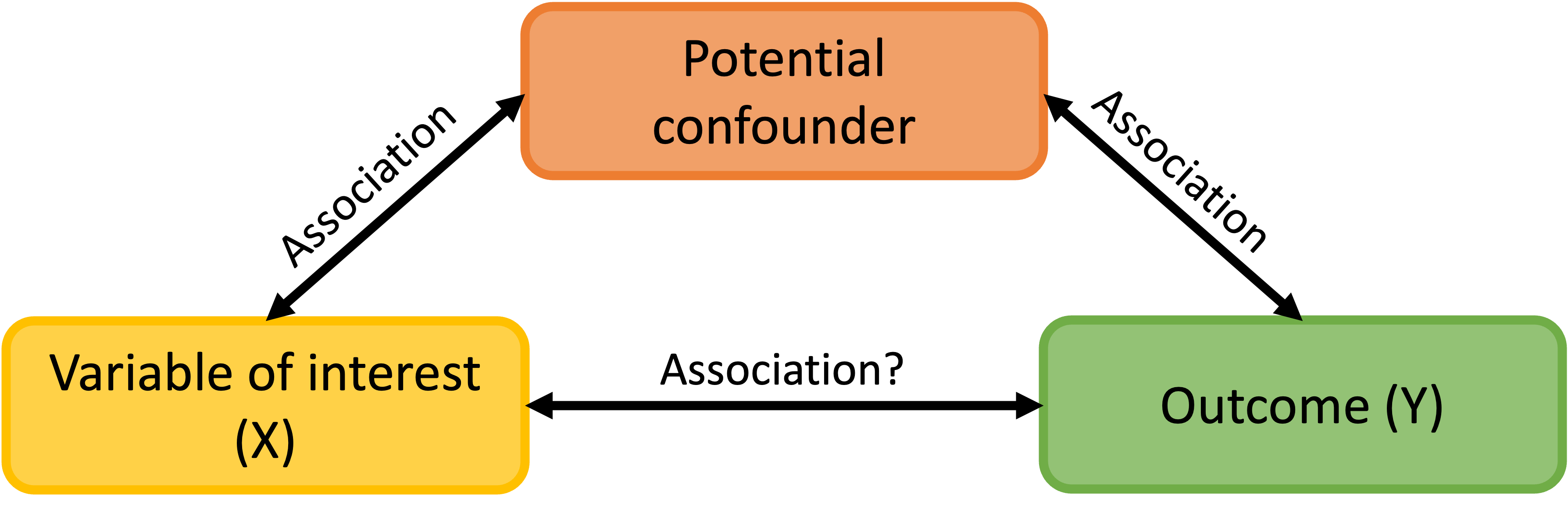
Revisit from 512/612: What is a confounder?
A confounding variable, or confounder, is a factor/variable that wholly or partially accounts for the observed effect of the risk factor on the outcome
A confounder must be…
- Related to the outcome Y, but not a consequence of Y
- Related to the explanatory variable X, but not a consequence of X
In study that does not meet causal assumptions (retrospective, observational, case-control)…
- We need to adjust for potential confounders
- We have no way of proving if a variable is a true confounder
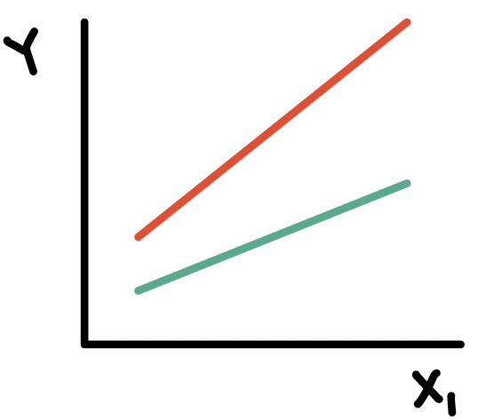
What is an effect modifier?
An additional variable in the model
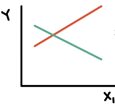
- Outside of the main relationship between \(Y\) and \(X_1\) that we are studying
An effect modifier will change the effect of \(X_1\) on \(Y\) depending on its value
Aka: as the effect modifier’s values change, so does the association between \(Y\) and \(X_1\)
So the coefficient estimating the relationship between \(Y\) and \(X_1\) changes with another variable
Example of interaction
- In a cohort study of elderly people the chance of death (outcome) within 2 years was much higher for those who had previously suffered a hip fracture at the start of these 2 years, but the excess risk associated with a hip fracture was significantly higher for males vs. females
- This is an interaction between hip fracture status (yes/no) and sex (unclear if assigned at birth or no)
- Odds ratio for females > odds ratio for males

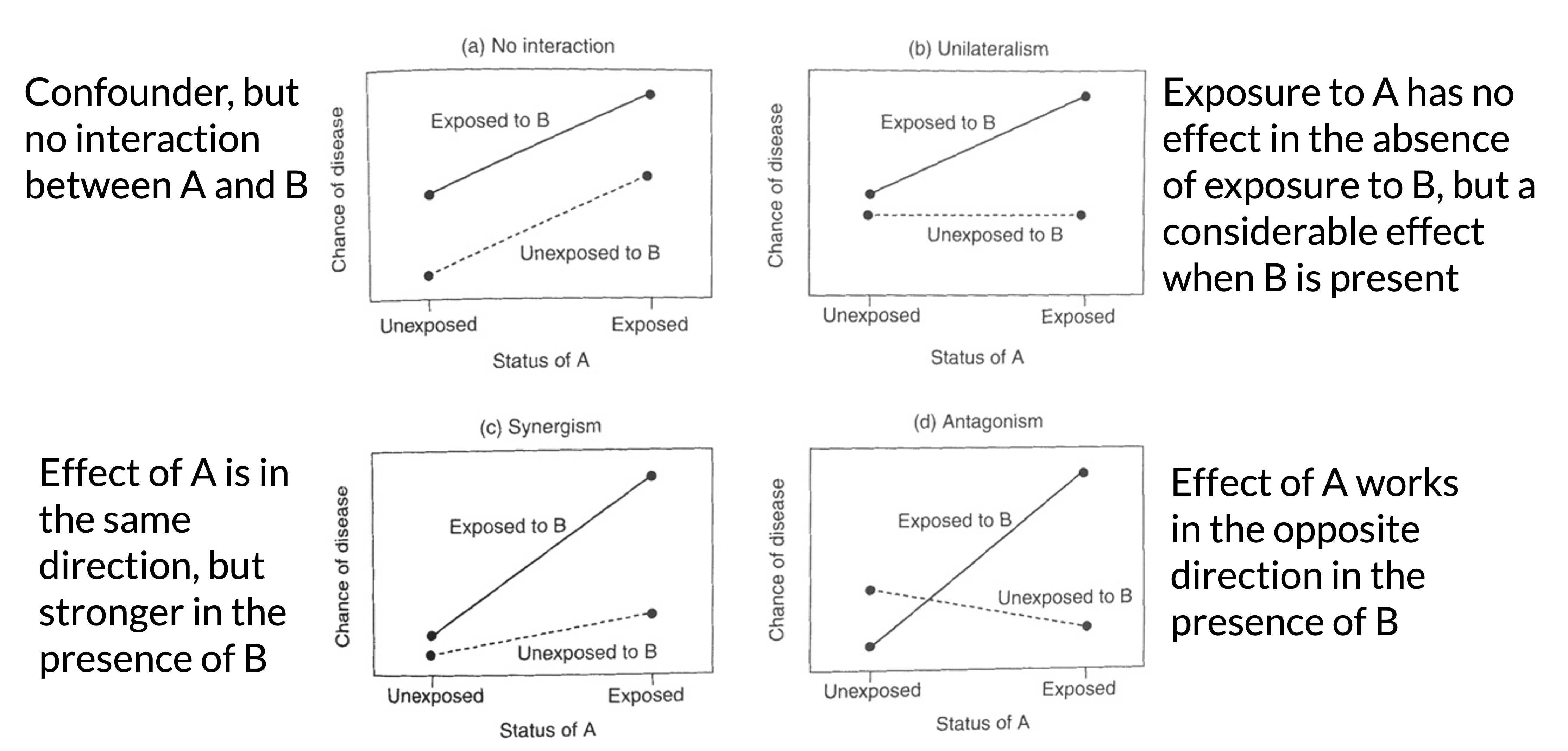
Types of interactions / non-interactions
Understand the interaction (1/3)
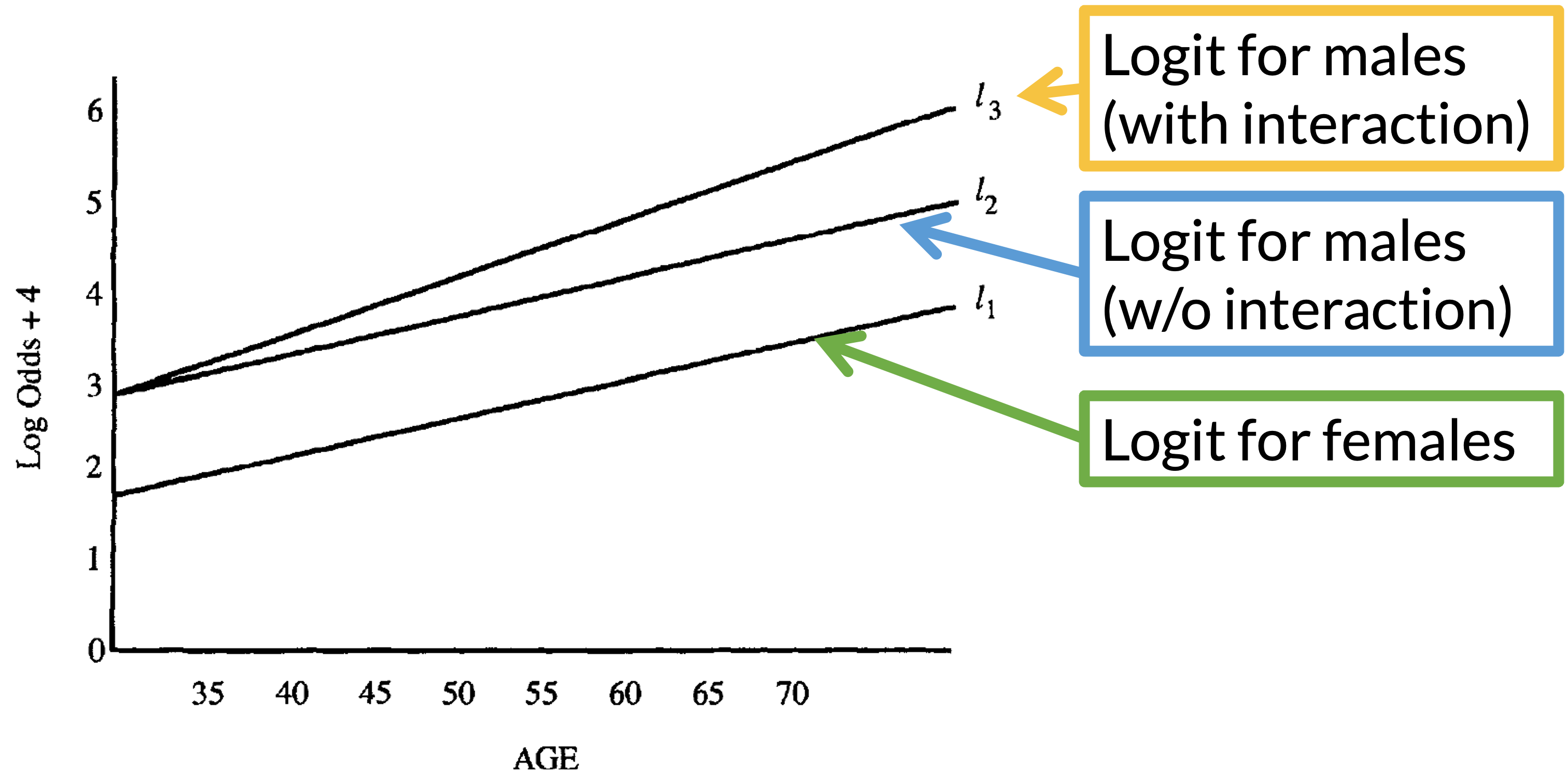
- Figure plots the logits (log-odds) under two different models:
- Model 1: No interaction between sex and age
- Model 2: Interaction between sex and age
- Response variable: CHD
- Risk factor: sex
- Covariate to be controlled: age
Understand the interaction (2/3)
- If age does not interact with sex, the distance between \(l_2\) and \(l_1\) is the log odds ratio for sex, controlling for age (\(l_2 - l_1\)) stays the same for all values of age.
If age interacts with sex, the distance between \(l_3\) and \(l_1\) is the log odds ratio for sex, controlling for age.
Age values need to be specified because (\(l_3 - l_1\)) differs for different values of age.
Must specify age when reporting odds ratio comparing sex
Understand the interaction (3/3)
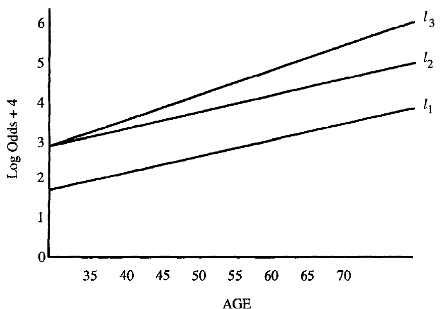
In the real world, it is rare to see two completely parallel logit plots as we see \(l_2\) and \(l_1\)
- But we need to determine if the difference between \(l_2\) and \(l_3\) is important in the model
- We may not want to include the interaction term unless it is statistically significant and/or clinically meaningful
- Likelihood ratio test (or Wald test sometimes) may be used to test the significance of an interaction term
Example: GLOW Study: Plot the proportions
ggplot(data = glow2, aes(y = freq, x = age, color = priorfrac)) +
  geom_point() + ylim(0, 1) + geom_smooth(se = F) +
  labs(x = "Age (years)", y = "Proportion of fracture",
       color = "Prior fracture", title = "Sample proportion of fracture by age and prior fracture") +
  theme(axis.title = element_text(size = 18), axis.text = element_text(size = 18),
        title = element_text(size = 18), legend.text=element_text(size=18))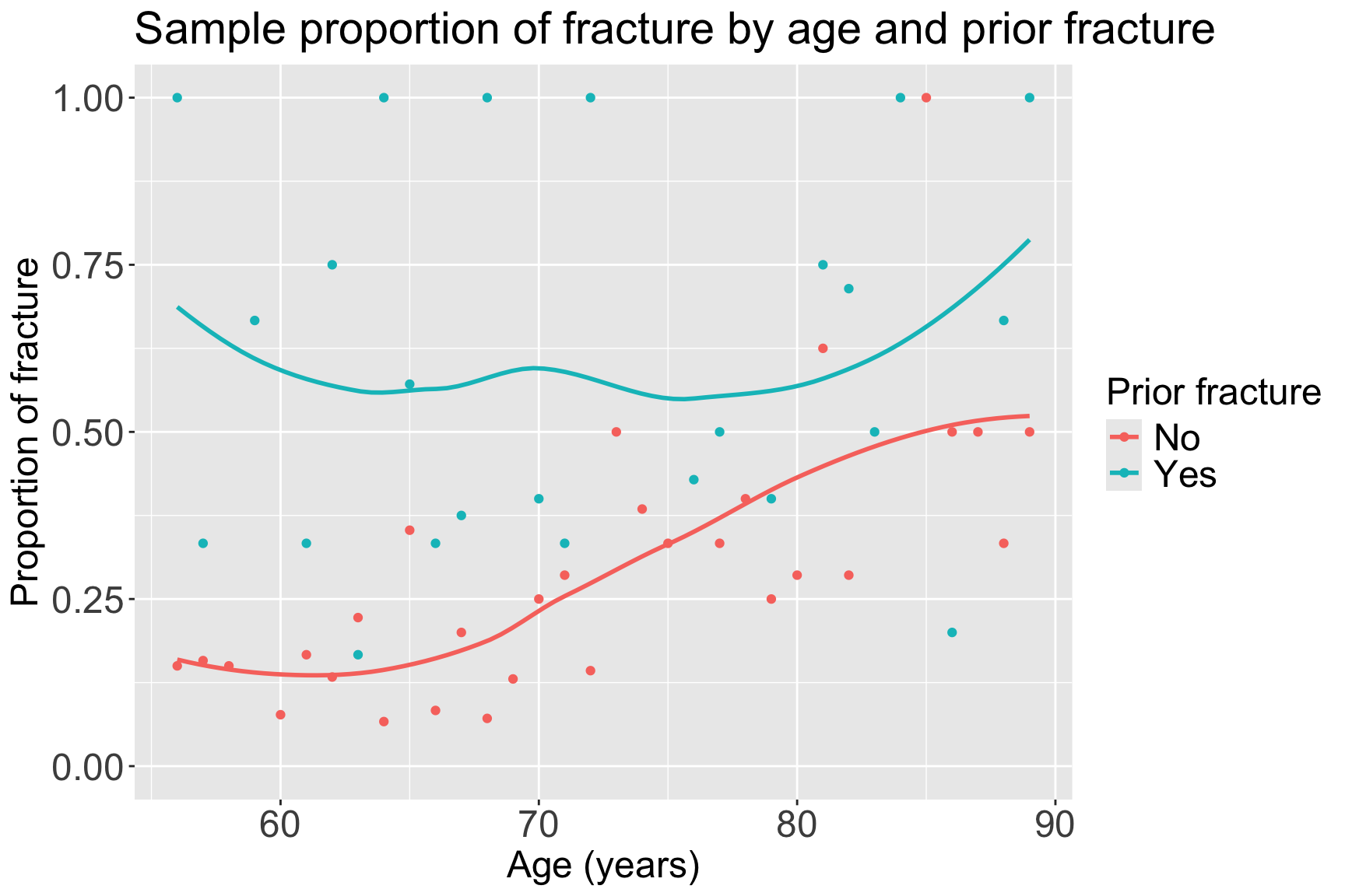
- From sample proportions, looks like age and prior fracture may have an interaction!
Plot of estimated log odds
prior_age = expand_grid(priorfrac = c("No", "Yes"), age_c = (55:90)-69)
frac_pred_log = predict(glow_m3, prior_age, se.fit = T, type="link")
pred_glow2 = prior_age %>% mutate(frac_pred_log = frac_pred_log$fit,
                                  age = age_c + mean_age)

ggplot(pred_glow2) + #geom_point(aes(x = age, y = frac_pred, color = priorfrac)) +
  geom_smooth(method = "loess", aes(x = age, y = frac_pred_log, color = priorfrac)) +
  theme(text = element_text(size=20), title = element_text(size=16)) +
  labs(color = "Prior Fracture", x = "Age (years)", y = "Log-Odds of Fracture")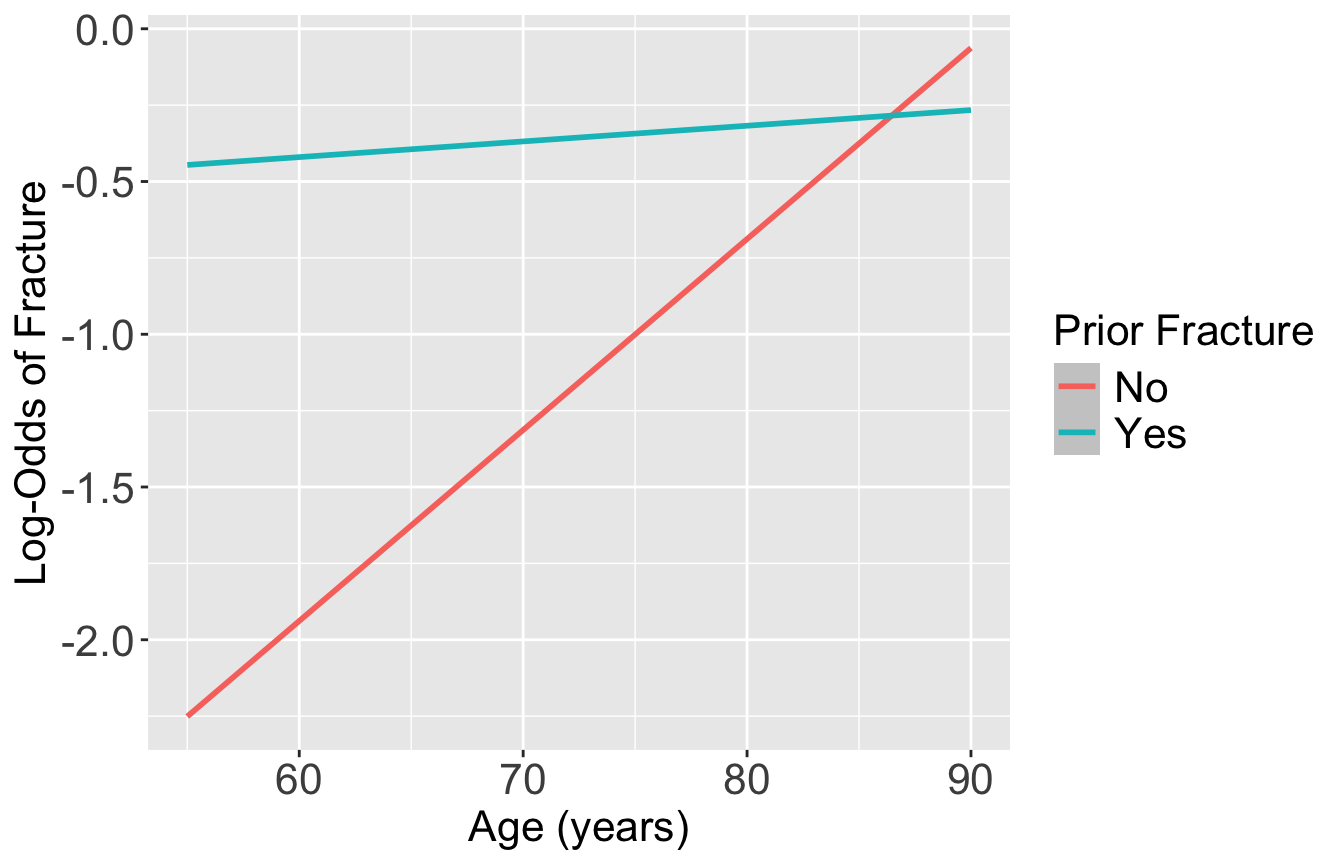
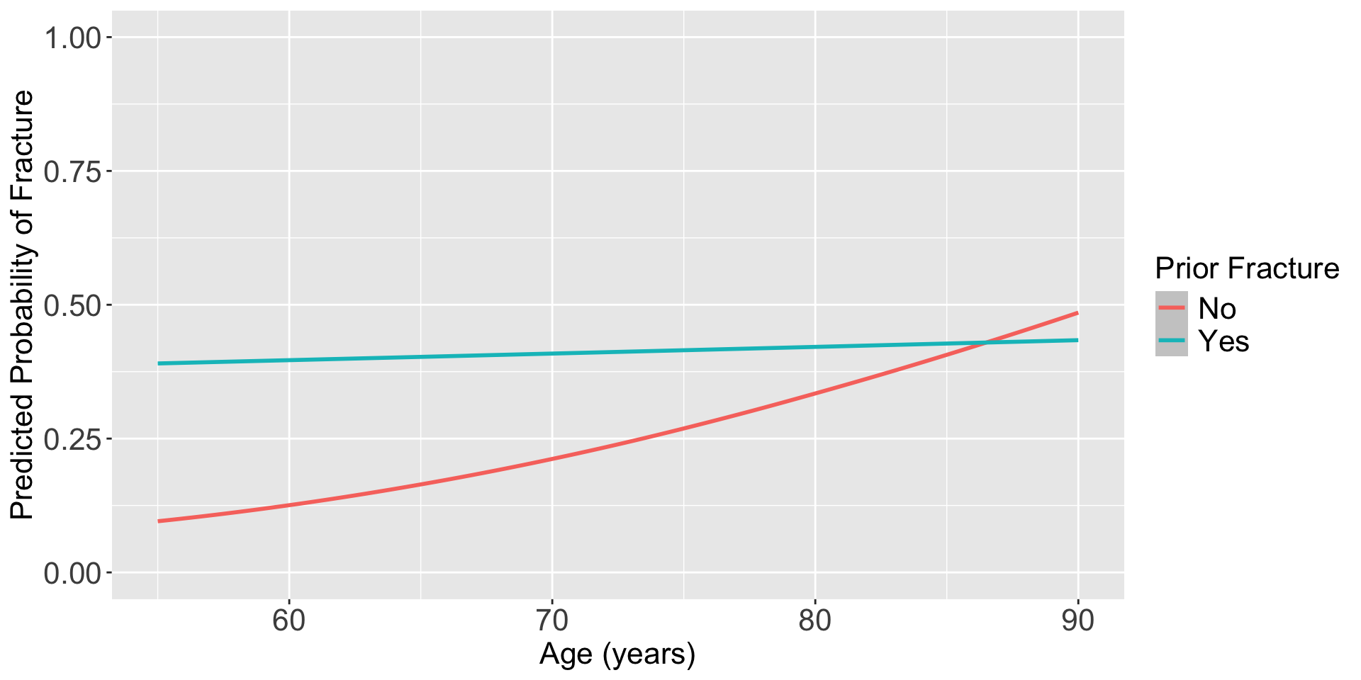
Plot the predicted probability of fracture
frac_pred = predict(glow_m3, prior_age, se.fit = T, type="response")
pred_glow = prior_age %>% mutate(frac_pred = frac_pred$fit,
                                  age = age_c + mean_age)

ggplot(pred_glow) + #geom_point(aes(x = age, y = frac_pred, color = priorfrac)) +
  geom_smooth(method = "loess", aes(x = age, y = frac_pred, color = priorfrac)) +
  theme(text = element_text(size=20), title = element_text(size=16)) + ylim(0,1) +
  labs(color = "Prior Fracture", x = "Age (years)", y = "Predicted Probability of Fracture")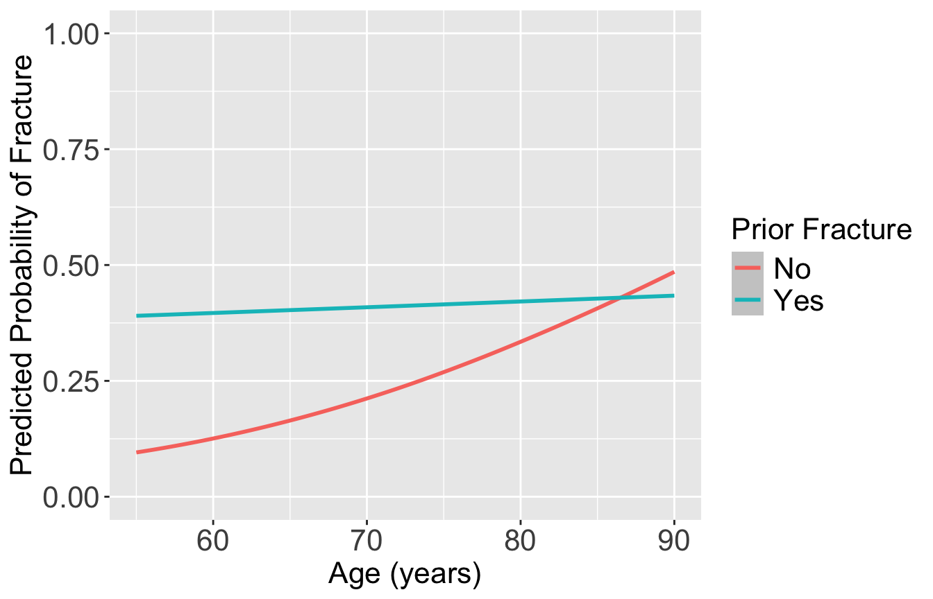
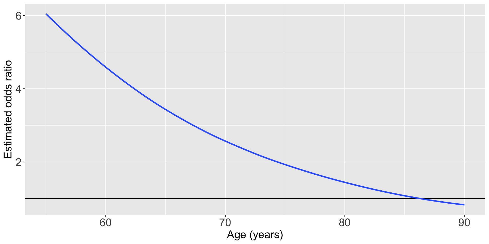
Plotting the odds ratio for an interaction
ggplot(pred_glow2) +
  geom_hline(yintercept = 1) +
  geom_smooth(method = "loess", aes(x = age, y = OR_YN)) +
  theme(text = element_text(size=20), title = element_text(size=16)) +
  labs(x = "Age (years)", y = "Estimated odds ratio", title = "Odds ratio of fracture outcome comparing \n prior fracture to no prior fracture")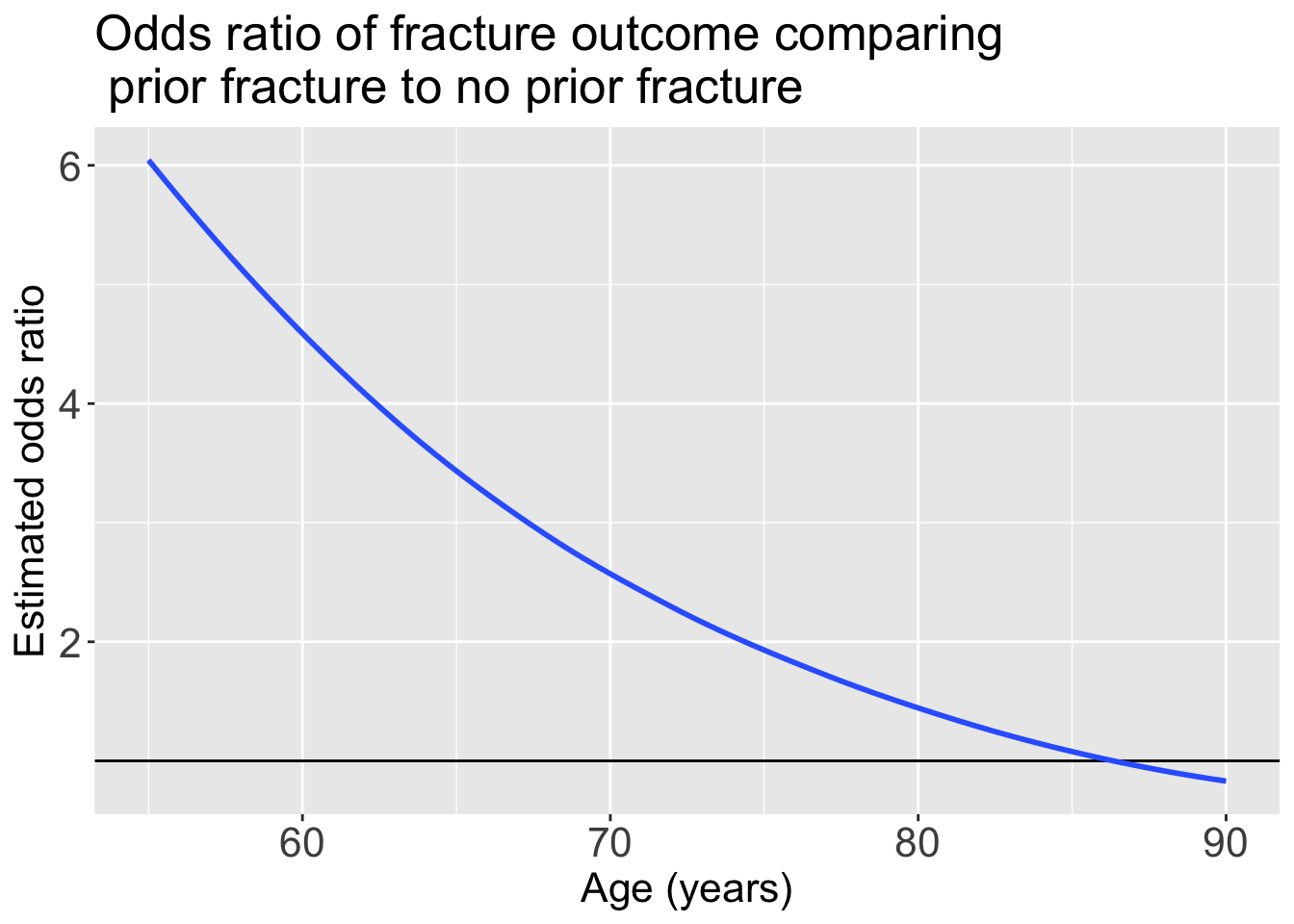
How would I report these results?
- Remember our main covariate is prior fracture, so we want to focuse on how age changes the relationship between prior fracture and a new fracture!
For individuals 69 years old, the estimated odds of a new fracture for individuals with prior fracture is 2.72 times the estimated odds of a new fracture for individuals with no prior fracture (95% CI: 1.70, 4.35). As seen in Figure 1 (a), the estimated odds ratio of a new fracture when comparing prior fracture status decreases with age, indicating that the effect of prior fractures on new fractures decreases as individuals get older. In Figure 1 (b), it is evident that for both prior fracture statuses, the predicted probability of a new fracture increases as age increases. However, the predicted probability of new fracture for those without a prior fracture increases at a higher rate than that of individuals with a prior fracture. Thus, the predicted probabilities of a new fracture converge at age [insert age here].