Lesson 13: Model Diagnostics
2025-05-12
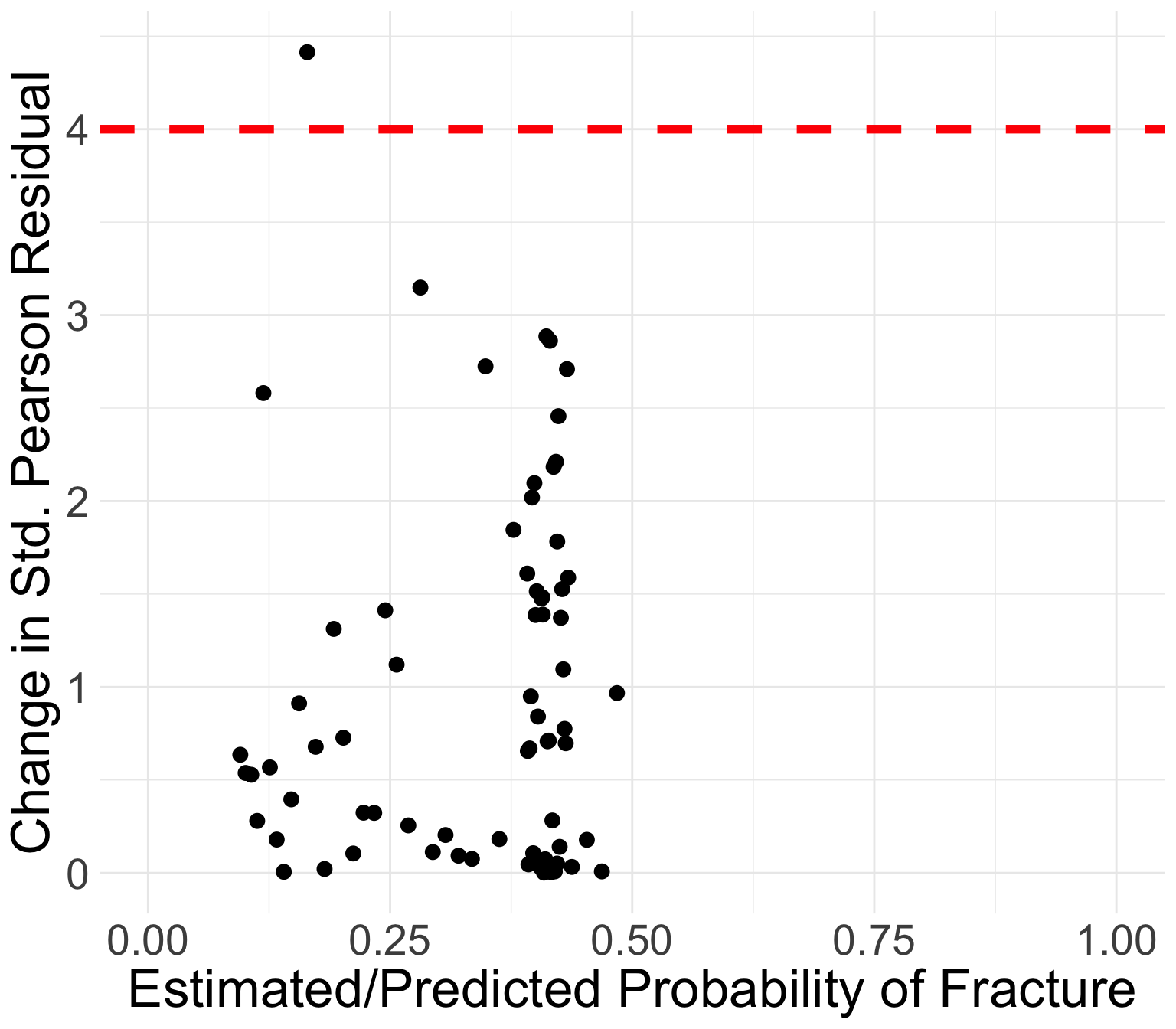
GLOW study: Change in standardized Pearson residuals
Generally, the points that curve from top left to bottom right of plot correspond to covariate patterns with \(Y_j = 1\)
- Opposite corresponds to \(Y_j = 0\)
Points in the top left or top right corners identify the covariate patterns that are poorly fit
We may use 4 as a crude approximation to the upper 95th percentile for \(\Delta X_j^2\)
- 95th percentile of chi-squared distribution is 3.84
Which point is over 4?

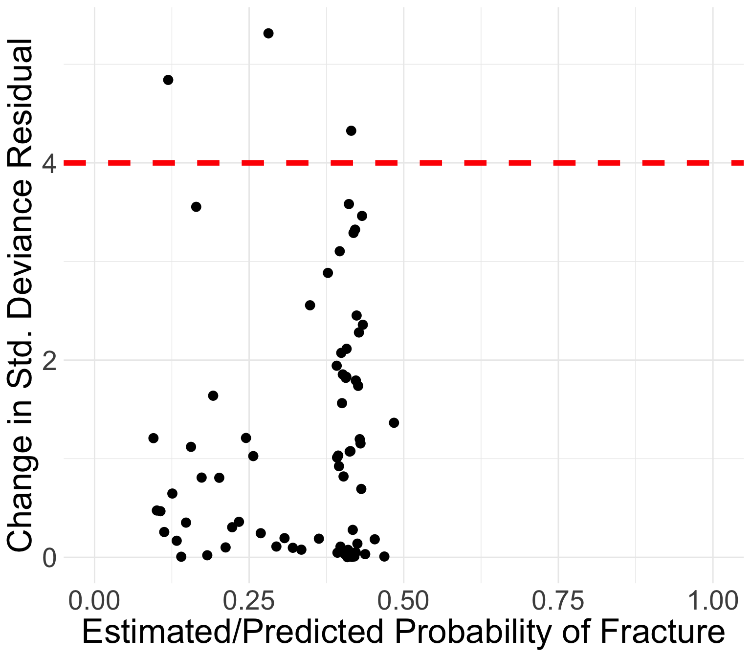
GLOW study: Change in standardized Deviance residuals
Same investigation as Pearson residuals
Points in the top left or top right corners identify the covariate patterns that are poorly fit
Use 4 as a crude approximation to the upper 95th percentile
Which point is over 4?
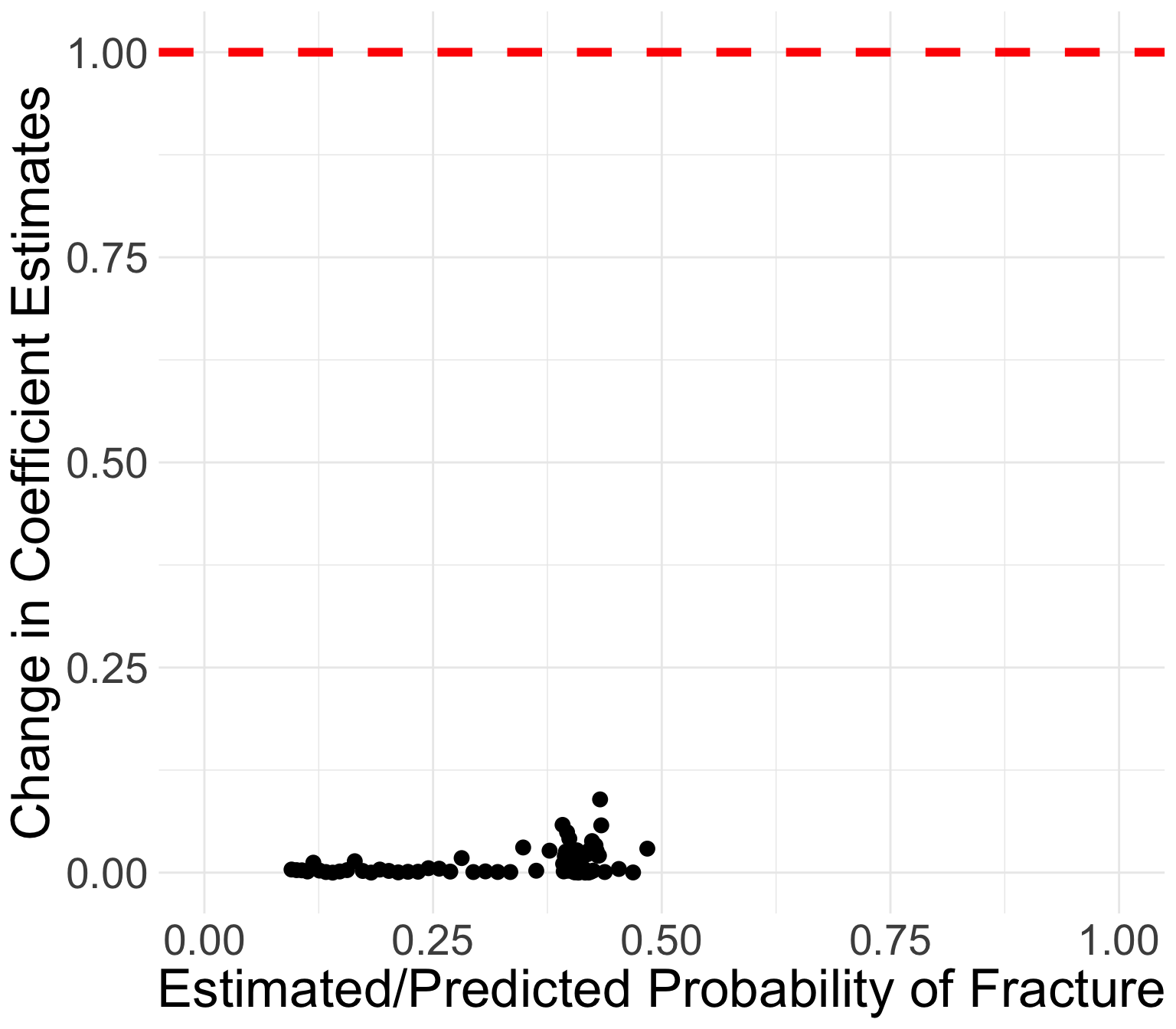
GLOW Study: Change in coefficient estimates
Book recommends flagging certain covariate patterns if change in coefficient estimates are greater than 1
All values of \(\Delta\widehat{\beta}_j\) are below 0.09
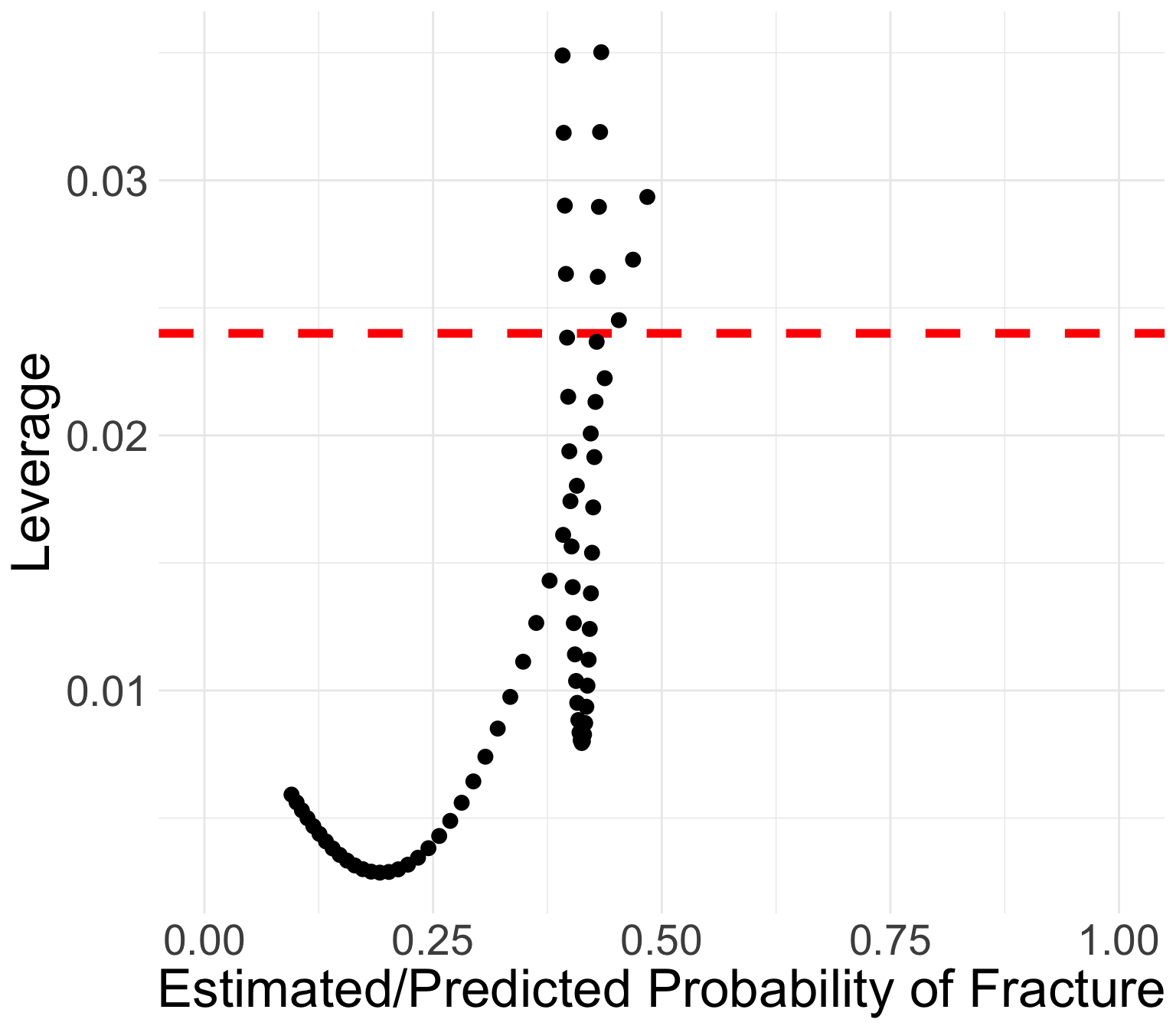
GLOW Study: Leverage
We can use the same rule as linear regression: \(h_j > 3p/n\)
- Flag these points as high leverage
Points with high leverage
- \(p=4\): four regression coefficients
- \(n=500\): 500 total observations
- Look for \(h_j > 3p/n = 3\cdot4 /500 = 0.024\)
   priorfracYes age_c         P          h
          <num> <num>     <num>      <num>
1:            0    20 0.4686423 0.02688958
2:            1   -12 0.3928116 0.03186122
3:            0    19 0.4531105 0.02451738
4:            1   -11 0.3940365 0.02900675
5:            1    19 0.4313389 0.02895824
6:            1    18 0.4300804 0.02621708