Chapter 14-20: Some Important Discrete RVs

Author

Meike Niederhausen and Nicky Wakim

Published

October 16, 2024

Learning Objectives

Distinguish between Bernoulli, Binomial, Geometric, Hypergeometric, Discrete Uniform, Negative Binomial, and Poisson distributions when reading a story.
Identify the variable and the parameters in a story, and state what the variable and parameters mean.
Use the formulas for the pmf/CDF, expected value, and variance to answer questions and find probabilities.

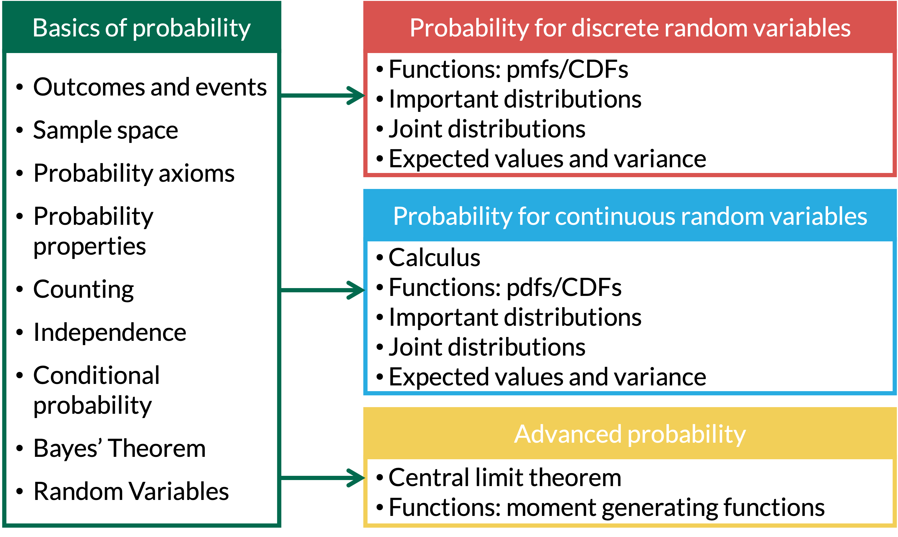
Where are we?

Chapter 14: Bernoulli RVs

Properties of Bernoulli RVs

Scenario: One trial, with outcome success or failure
Shorthand: $X \sim \text{Bernoulli}(p)$

\[ X = \left\{ \begin{array}{ll} 1 & \quad \mathrm{with\ probability}\ p \quad \\ 0 & \quad \mathrm{with\ probability}\ 1-p \quad \end{array} \right. \]

\[ p_X(x) = P(X=x) = p^x(1-p)^{1-x} \text{ for } x=0,1 \]

\[\text{E}(X) = p\]

\[\text{Var}(X) = pq = p(1-p)\]

Bernoulli Example 1

Example 1

We roll a fair 6-sided die.
We get $1 if we roll a 5, and nothing otherwise.
Let $X$ be how much money we get.
Find the mean and variance of $X$.

Chapter 15: Binomial RVs

Properties of Binomial RVs

Scenario: There are $n$ independent trials, each resulting in a success or failure, with constant probability, $p$, in each trial. We are counting the number of successes (or failures).
Shorthand: $X \sim \text{Binomial}(n, p)$

\[ X = \text{Number of successes of } n \text{ independent trials} \]

\[ p_X(x) = P(X=x) = {n \choose x}p^x(1-p)^{n-x} \text{ for } x=0,1,2, ..., n \]

\[\text{E}(X) = np\] \[\text{Var}(X) = npq = np(1-p)\]

Our beloved fair-sided die

Example 2

Suppose we roll a fair 6-sided die 50 times.
We get $1 every time we roll a 5, and nothing otherwise.
Let $X$ be how much money we get on the 50 rolls.
Find the mean and variance of $X$.

Chapter 16: Geometric RVs

Geometric RVs

Scenario: There are repeated independent trials, each resulting in a success or failure, with constant probability of success for each trial. We are counting the number of trials until the first success.
Shorthand: $X \sim \text{Geo}(p)$ or $X \sim \text{Geometric}(p)$ or $X \sim \text{G}(p)$

\(X =\) Number of trials needed for first success (count \(x\) includes the success)	\(X =\) Number of failures before first success (count \(x\) does not include the success)
\(p _ X( x ) = P(X=x) = (1-p)^{x-1}p\) for \(x=1,2, 3,...\) \[F_ X(x ) = P(X\leq x) = 1-(1-p)^x\] for \(x=1,2, 3,...\)	\(p _X (x)= P(X=x) = (1-p)^{x}p\) for \(x=0, 1,2,...\) \[F_X ( x ) = P(X\leq x) = 1-(1-p)^{x+1}\] for \(x=0, 1,2,...\)
\(E(X)=\dfrac{1}{p}\) \(Var(X)= \dfrac{1-p}{p^2}\)	\(E(X)=\dfrac{1-p}{p}\) \(Var(X) = \dfrac{1-p}{p^2}\)

$p _ X( x ) = P(X=x) = (1-p)^{x-1}p$

for $x=1,2, 3,...$

\[F_ X(x ) = P(X\leq x) = 1-(1-p)^x\]

for $x=1,2, 3,...$

$p _X (x)= P(X=x) = (1-p)^{x}p$

for $x=0, 1,2,...$

\[F_X ( x ) = P(X\leq x) = 1-(1-p)^{x+1}\]

for $x=0, 1,2,...$

$E(X)=\dfrac{1}{p}$

$Var(X)= \dfrac{1-p}{p^2}$

$E(X)=\dfrac{1-p}{p}$

$Var(X) = \dfrac{1-p}{p^2}$

Bullseye (1/4)

Example 3

We throw darts at a dartboard until we hit the bullseye. Assume throws are independent and the probability of hitting the bullseye is 0.01 for each throw.

What is the pmf for the number of throws needed to hit the bullseye?
What are the mean and variance for the number of throws needed to hit the bullseye?
Find the probability that our first bullseye:
- is on one of the first fifty tries
- is after the $50^{th}$ try, given that it did not happen on the first 20 tries

Bullseye (2/4)

Example 3

We throw darts at a dartboard until we hit the bullseye. Assume throws are independent and the probability of hitting the bullseye is 0.01 for each throw.

What is the pmf for the number of throws needed to hit the bullseye?

Bullseye (3/4)

Example 3

We throw darts at a dartboard until we hit the bullseye. Assume throws are independent and the probability of hitting the bullseye is 0.01 for each throw.

What are the mean and variance for the number of throws needed to hit the bullseye?

Bullseye (4/4)

Example 3

We throw darts at a dartboard until we hit the bullseye. Assume throws are independent and the probability of hitting the bullseye is 0.01 for each throw.

Find the probability that our first bullseye:
- is on one of the first fifty tries
- is after the $50^{th}$ try, given that it did not happen on the first 20 tries

Memoryless property for Geometric RVs

If we know $X$ is greater than some number (aka given $X >j$), then the probability of $X > k+j$ is just the probability that $X>k$.

$P(X > k+j |X > j) = P(X > k)$ \[ P(X > k+j |X > j) = \dfrac{P(X>k+j \text{ and } X>j)}{P(X>j)} = \dfrac{P(X>k+j)}{P(X>j)} = \dfrac{(1-p)^{k+j}}{(1-p)^{j}} = (1-p)^{k} \]

Chapter 17: Negative Binomial RVs

Properties of Negative Binomial RVs

Scenario: There are repeated independent trials, each resulting in a success or failure, with constant probability of success for each trial. We are counting the number of trials until the $r^{th}$ success.
Shorthand: $X \sim \text{NegBin}(p, r)$ or $X \sim \text{NB}(p, r)$
Negative binomial is sum of $r$ geometric distributions

\[ X = \text{Number of independent trials until } r^{th} \text{ success} \]

\[ p_X(x) = P(X=x) = {x-1 \choose r-1}(1-p)^{x-r}p^r \text{ for } x = r, r+1, r+2, ...\]

\[ E(X) = \dfrac{r}{p}\]

\[Var(X) = \dfrac{rq}{p^2} = \dfrac{r(1-p)}{p^2}\]

Hitting more than 1 bullseye

Example 1

Consider again the bullseye example, where we throw darts at a dartboard until we hit the bullseye. Assume throws are independent and the probability of hitting the bullseye is 0.01 for each throw.

What is the expected value and variance of the number of throws needed to hit 5 bullseyes?

Hitting more than 1 bullseye

Example 1

Consider again the bullseye example, where we throw darts at a dartboard until we hit the bullseye. Assume throws are independent and the probability of hitting the bullseye is 0.01 for each throw.

What is the probability that the $5^{th}$ bullseye is on the $20^{th}$ throw?

5 minute break

Chapter 18: Poisson RVs

Properties of Poisson RVs

Scenario: We are counting the number of successes in a fixed time period, which has a constant rate of successes
Shorthand: $X \sim \text{Poisson}(\lambda)$ or $X \sim \text{Pois}(\lambda)$

\[ X = \text{Number of successes in a given period} \]

\[ p_X(x) = P(X=x) = \dfrac{e^{-\lambda}\lambda^x}{x!} \text{ for } x = 0, 1, 2,3, ...\]

\[ \text{E}(X) = \lambda\]

\[\text{Var}(X) = \lambda\]

Distinguishing between Binomial and Poisson RVs

Recall that if $X\sim \text{Binomial}(n,p)$, then
- $X$ models the number of successes …
- in $n$ independent (Bernoulli) trials …
- that each have the same probability of success $p$.
Poisson r.v.’s are similar,
- except that instead of having $n$ discrete independent trials,
- there is a fixed time period (or space) during which the successes happen

Examples of Poisson RVs

Number of visitors to an emergency room in an hour during a weekend night
Number of study participants enrolled in a study per week
Number of pedestrians walking through a square mile
Any more?

Emergency Room Visitors

Example 1

Suppose an emergency room has an average of 50 visitors per day. Find the following probabilities.

Probability of 30 visitors in a day.
Probability of 8 visitors in an hour.
Probability of at least 8 visitors in an hour.

Combining independent Poisson distributions

Theorem 1

If $X\sim Pois(\lambda_1)$ and $Y\sim Pois(\lambda_2)$ are independent of each other, then $Z=X+Y\sim Pois(\lambda_1 + \lambda_2)$.

Two emergency rooms

Example 2

Suppose emergency room 1 has an average of 50 visitors per day, and emergency room 2 has an average of 70 visitors per day, independently of each other. What is the probability distribution to model of the total number of visitors to both?

Poisson Approximation of the Binomial

Both Poisson and Binomial r.v.’s are counting the number of successes

If for a Binomial r.v.
- the number of trials $n$ is very large, and
- the probability of success $p$ is close to 0 or 1,
Then the Poisson distribution can be used to approximate Binomial probabilities
- and we use $\lambda = np$
Rule of thumb: We can use the Poisson approximation when $\dfrac{1}{10} \leq np(1-p) \leq 10$

Medical lab errors

Example 3

Suppose that in the long run, errors in a medical testing lab are made 0.1% of the time. Find the probability that fewer than 4 mistakes are made in the next 2,000 tests.

Find the probability using the Binomial distribution.
Approximate the probability in part (1) using the Poisson distribution.

To do for extra practice - will also see a similar problem in BSTA 511

Chapter 19: Hypergeometric RVs

Hypergeometric RVs

Scenario: There are a fixed number of successes and failures (which are known in advance), from which we make $n$ draws without replacement. We are counting the number of successes from the $n$ trials.
- There is a finite population of $N$ items
- Each item in the population is either a success or a failure, and there are $M$ successes total.
- We randomly select (sample) $n$ items from the population without replacement
Shorthand: $X \sim \text{Hypergeo}(M, N, n)$

\[ X = \text{Number of successes in } n \text{ draws} \]

\[ p_X(x) = P(X=x) = \dfrac{{M \choose x}{N-M \choose n-x}}{{N \choose n}} \] \[\text{ for } x \text{ integer-valued } \\ \max(0, n-(N-M)) \leq x \leq \min(n, M)\]

\[\text{E}(X) =\dfrac{nM}{N}\]

\[\text{Var}(X) = n \dfrac{M}{N} \bigg(1- \dfrac{M}{N} \bigg)\bigg(\dfrac{N-n}{N-1} \bigg)\]

Wolf population

Example 4

A wildlife biologist is using mark-recapture to research a wolf population. Suppose a specific study region is known to have 24 wolves, of which 11 have already been tagged. If 5 wolves are randomly captured, what is the probability that 3 of them have already been tagged?

Binomial approximation of the hypergeometric RV

Suppose a hypergeometric RV $X$ has the following properties:

the population size $N$ is really big,
the number of successes $M$ in the population is relatively large,
- $\frac{M}{N}$ shouldn’t be close to 0 or 1
and the number of items $n$ selected is small
Rule of thumb: $\dfrac{n}{N}<0.05$ or $N>20n$

Then, in this case, making $n$ draws from the population doesn’t change the probability of success much, and the hypergeometric RV. can be approximated by a binomial RV

Wolf population revisited

Example 5

Suppose a specific study region is known to have 2400 wolves, of which 1100 have already been tagged.

If 50 wolves are randomly captured, what is the probability that 20 of them have already been tagged?
Approximate the probability in part (1) using the binomial distribution.

Chapter 20: Discrete Uniform RVs

Discrete Uniform RVs

Scenario: There are $N$ possible outcomes, which are all equally likely.
Shorthand: $X \sim \text{Uniform}(N)$

\[ X = \text{Outcome of interest, with } x=1, 2, ..., N \]

\[ p_X(x) = P(X=x) = \dfrac{1}{N} \text{ for } x=1, 2, 3, ..., N \]

\[\text{E}(X) =\dfrac{N+1}{2}\]

\[\text{Var}(X) = \dfrac{N^2 -1}{12}\]

What discrete uniform RVs have we seen already?

Example 6

Examples of discrete uniform RVs