Muddy Points

Chapter 12: Variance of Discrete RVs

Muddy Points from Fall 2023:

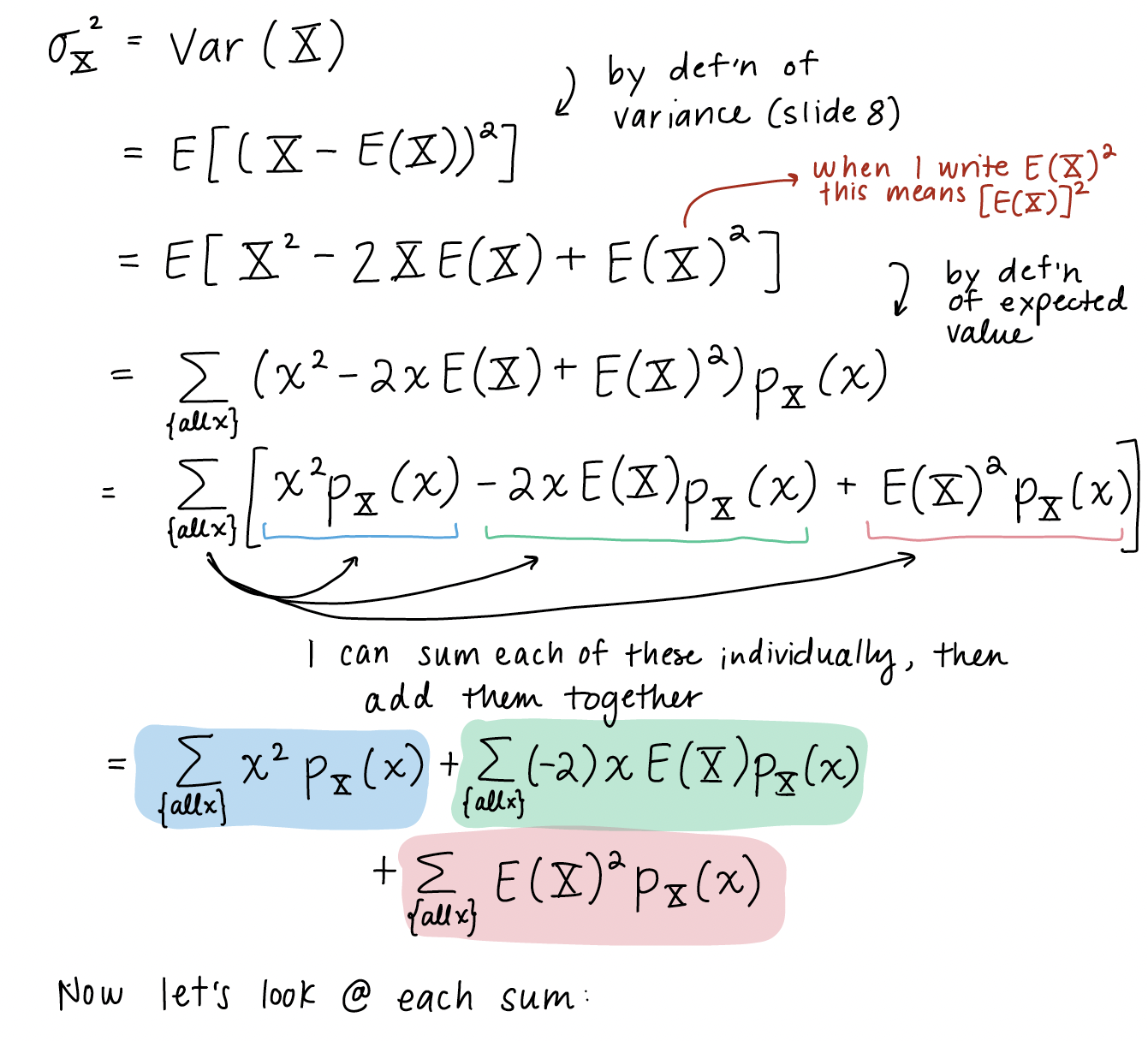
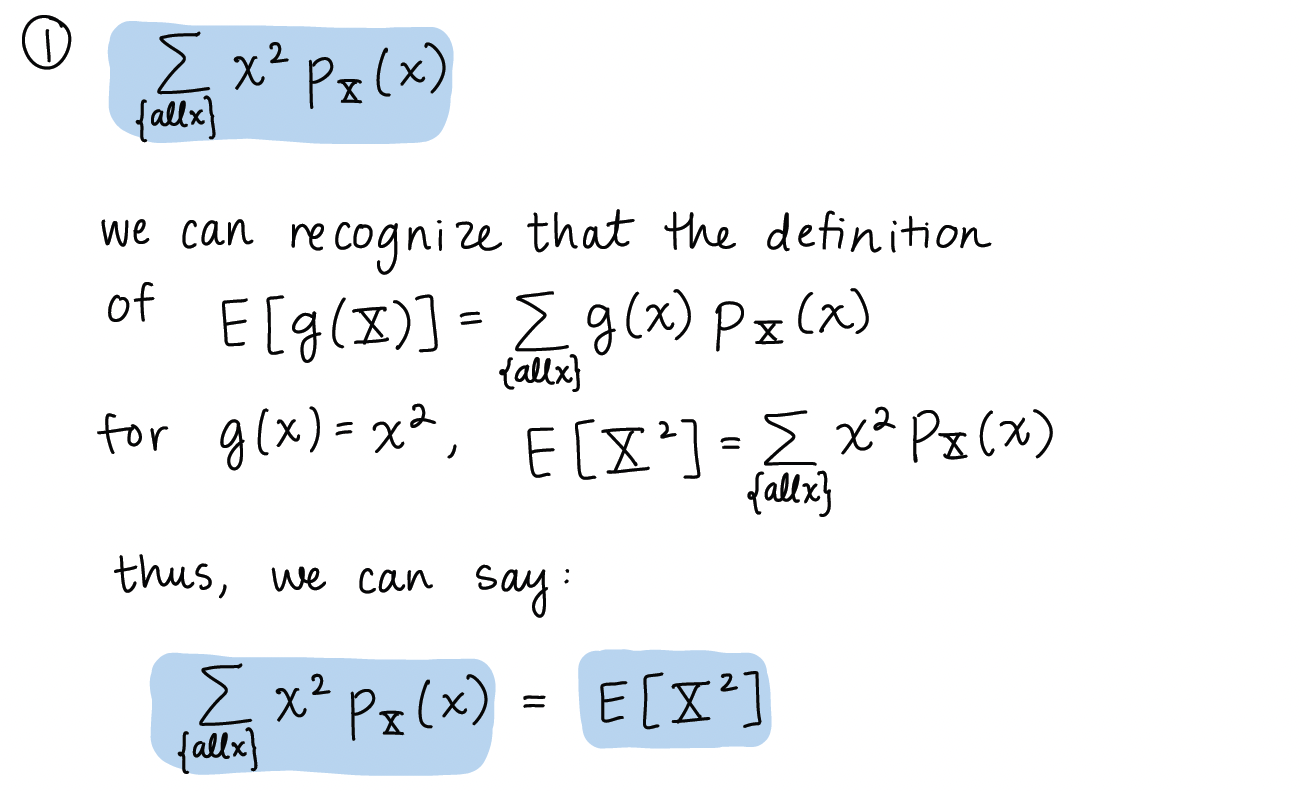
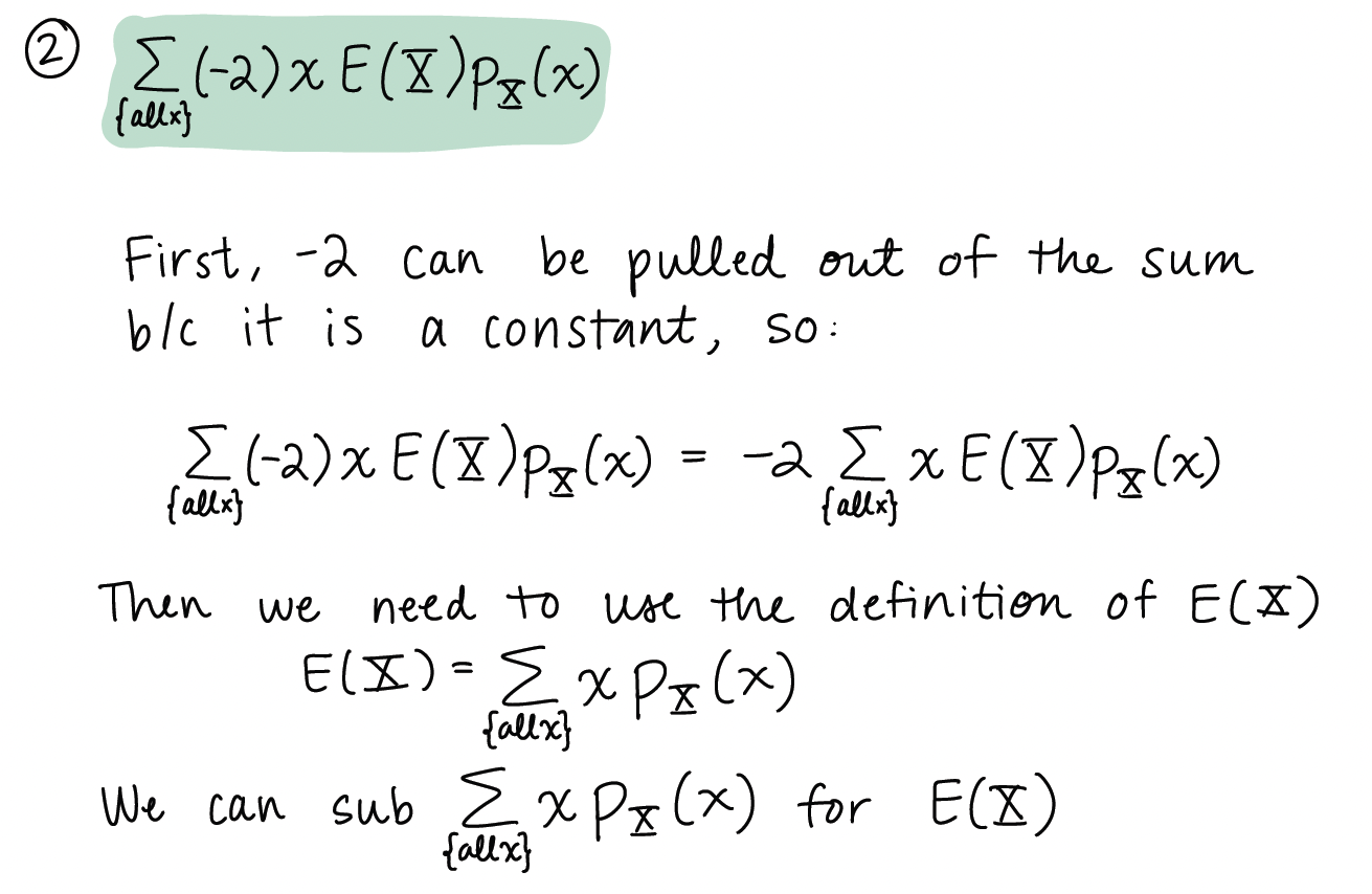
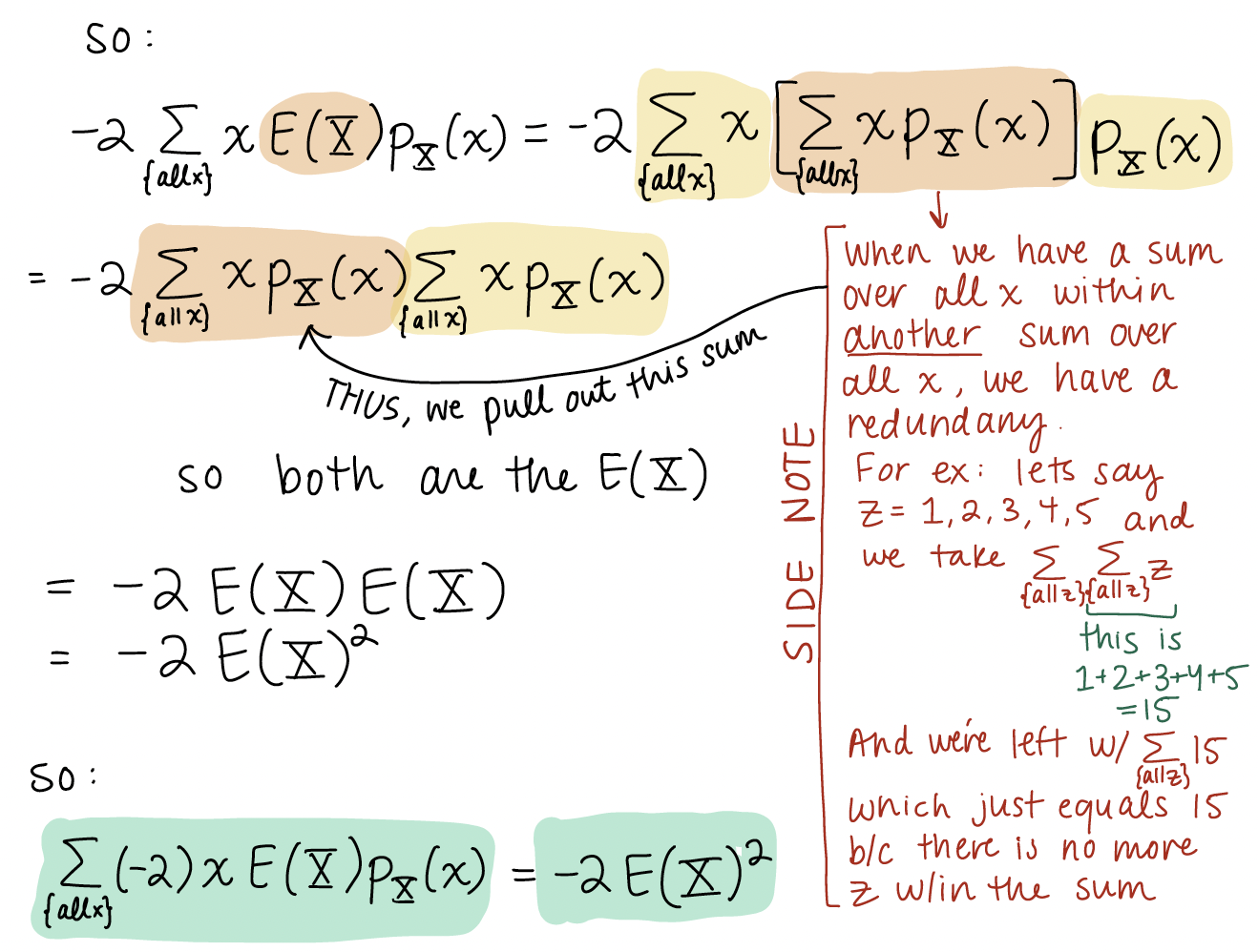
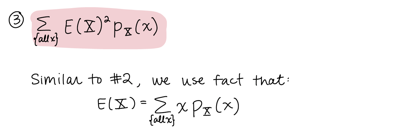
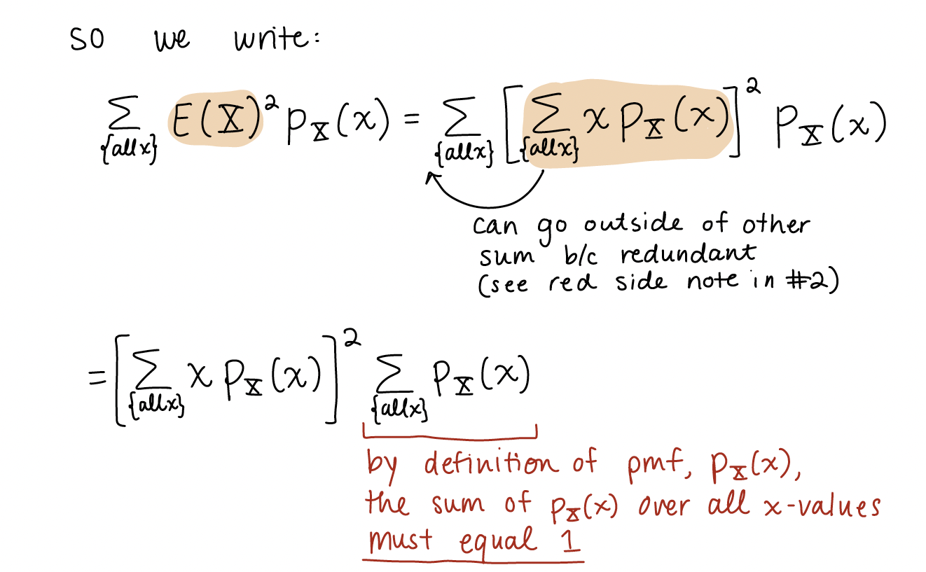
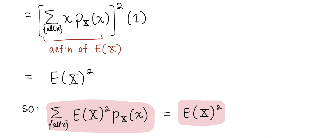
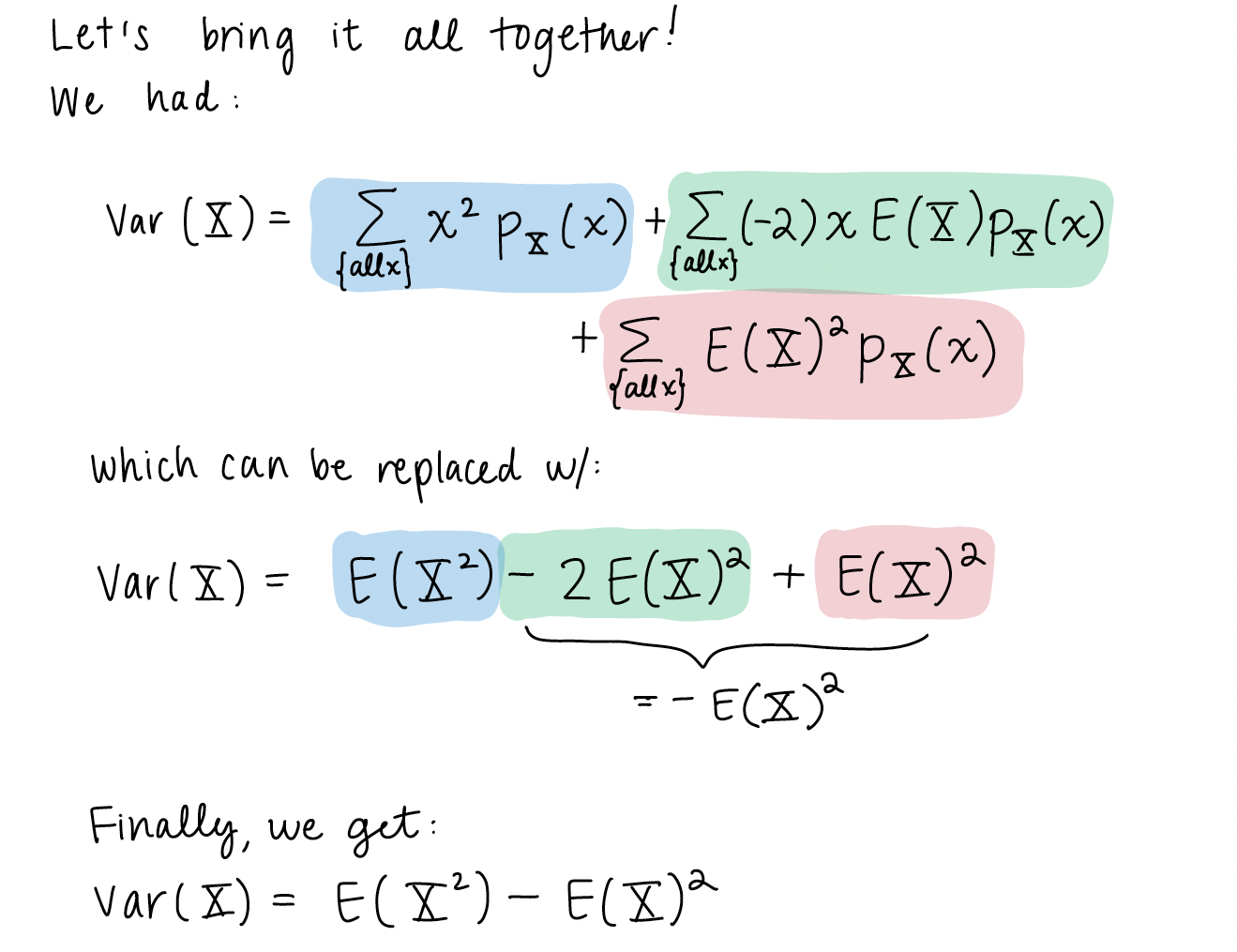
1. Proof of variance formula

Here is the variance formula that we worked through on slide 9 of Chapter 12’s notes.

Lemma 6: “Computation formula” for variance

The variance of a r.v. \(X\), can be computed as \[\begin{align}\sigma_X^2 & =Var(X) \\ & = \mathbb{E}[X^2]-\mu_X^2 \\ & = \mathbb{E}[X^2] - (\mathbb{E}[X])^2\end{align}\]

I stepped through this quite quickly and made some implicit steps. So let’s revisit it with explicit steps!

2. What progression are we following in the course??

Someone asked if this is our progression: RV is function \(\to\) Expected value is function to describe mean of RV \(\to\) Use functions within expected value to set up variance

Basically, yes! The random variable is a function of a random process. The RV inherits that randomness.

From there, we’ve been working towards calculating the probability of a realized value ($x$) of the RV. The probability can be different for different realized values (as it links back to the random process).

We also want to construct ways to describe our random variables. We may want to figure out what to expect from our random variable (which translates to the mean value of the RV). Since our RV is rooted in a random process, we may want to get an idea of how spread out our realized values are. We use our expected value (mean) as an anchor in our spread. Variance is one way to measure this spread.