library("ggplot2")
eq = function(x){(1/9)*x^2}
ggplot(data.frame(x=c(1, 50)), aes(x=x)) +
  stat_function(fun=eq) +
  xlab("x") + ylab("pdf") +
  xlim(0,3)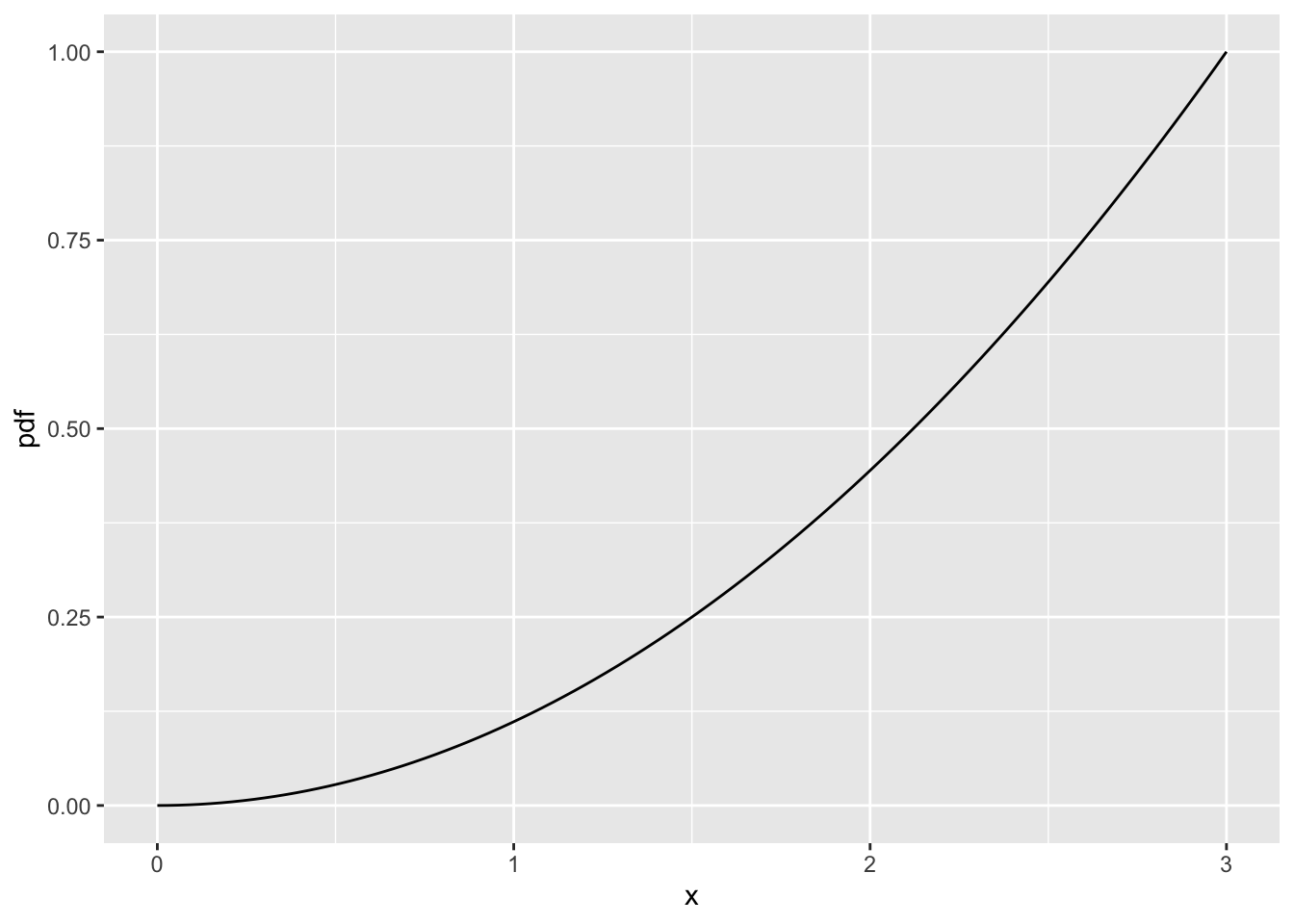
Chapter 25: Joint densities
November 20, 2024
November 25, 2024
Muddy points from Fall 2023:
Let’s say we have a pdf, \(f_X(x) = \dfrac{1}{9}x^2\) for \(0 \leq x \leq 3\). This is just a function. The pdf is not used on its own to report any probability. We must integrate over the pdf to find a probability.
library("ggplot2")
eq = function(x){(1/9)*x^2}
ggplot(data.frame(x=c(1, 50)), aes(x=x)) +
stat_function(fun=eq) +
xlab("x") + ylab("pdf") +
xlim(0,3)
The total area under the pdf is 1. This makes our pdf valid.
eq = function(x){(1/9)*x^2}
ggplot(data.frame(x=c(1, 50)), aes(x=x)) +
  stat_function(fun=eq) +
  xlab("x") + ylab("pdf") +
  xlim(0,3) +
  stat_function(fun=eq,
                xlim = c(0, 3),
                geom = "area",
                aes(fill = "red")) +
  theme(legend.position = "none") +
  annotate("text", x = 0.5, y = 0.7, label = "AUC = 1", color = "black")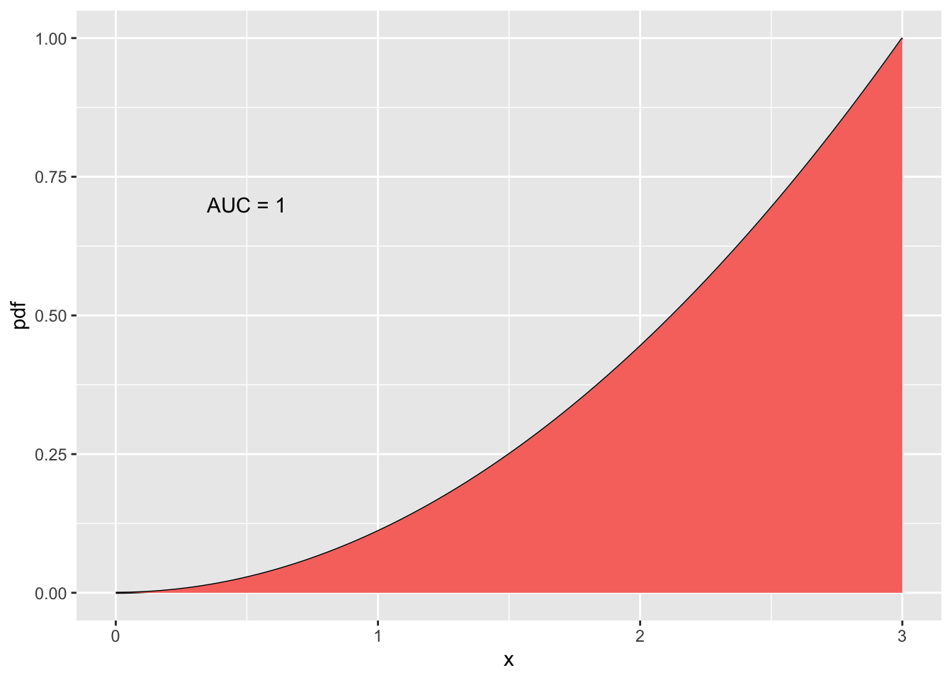
If we only look at a proportion of the area under the pdf, then we start constructing our probabilities. For example, we can look at probability that we have a value between 0 and 1.5.
ggplot(data.frame(x=c(1, 50)), aes(x=x)) +
  stat_function(fun=eq) +
  xlab("x") + ylab("pdf") +
  xlim(0,3) +
  stat_function(fun=eq,
                xlim = c(0, 1.5),
                geom = "area",
                aes(fill = "blue")) +
  theme(legend.position = "none") +
  annotate("text", x = 0.5, y = 0.7, label = "AUC = 0.125", color = "black")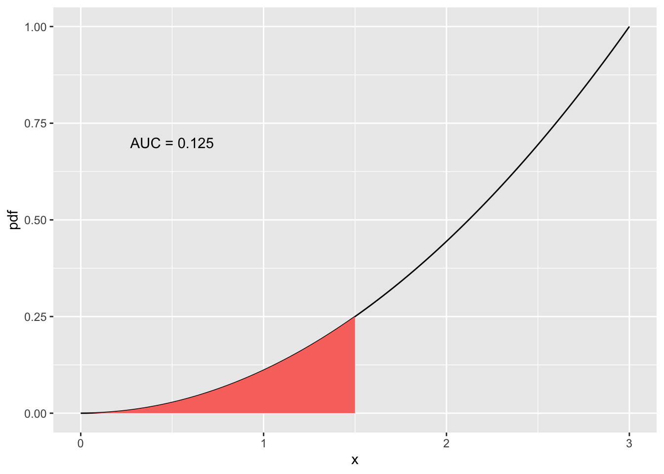
Instead of calculating the EXACT probability for each value between 0 and 3, we can find the CDF of the pdf.
The CDF is: \[ F_X(x) = \left\{ \begin{array}{ll} 0 & \quad x<3 \quad \\ \dfrac{1}{27}x^3 & \quad 0 \leq x \leq 3\quad \\ 1 & \quad x>3 \quad \end{array} \right. \]
cdf = function(x){(1/27)*x^3}
ggplot(data.frame(x=c(1, 50)), aes(x=x)) +
  stat_function(fun=cdf) +
  xlab("x") + ylab("CDF") +
  xlim(0,3) +
  theme(legend.position = "none")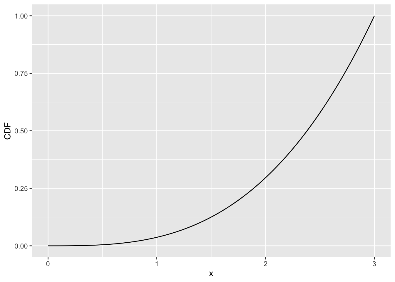
When \(x=1.5\), we can calculate the probability using the CDF. Remember that \(F_X(x) = P(X \leq x)\). So we can say \(P(X \leq 1.5) = F_X(1.5) = \dfrac{1}{27}(1.5)^3\), which equals 0.125.
cdf = function(x){(1/27)*x^3}
ggplot(data.frame(x=c(1, 50)), aes(x=x)) +
  stat_function(fun=cdf) +
  xlab("x") + ylab("CDF") +
  xlim(0,3) +
  theme(legend.position = "none") +
  geom_point(aes(x=1.5, y=.125), colour="blue", size=3) +
  annotate("text", x = 0.5, y = 0.7, label = "CDF = 0.125", color = "black")
Warning in geom_point(aes(x = 1.5, y = 0.125), colour = "blue", size = 3): All aesthetics have length 1, but the data has 2 rows.
ℹ Please consider using `annotate()` or provide this layer with data containing
a single row.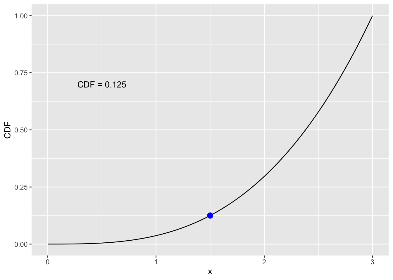
We can also calculate the probability with an integral: \(P(X \leq 1.5) = \displaystyle\int_0^{1.5} \dfrac{1}{9}x^2 dx\).
We can also find the probability that X is between two numbers. \(P(1\leq X \leq 1.5) = F_X(1.5) - F_X(1)\) or \(P(1\leq X \leq 1.5) = \displaystyle\int_1^{1.5} \dfrac{1}{9}x^2 dx\).
If we start at a joint probability \(f_{X,Y}(x,y)\)…. we can look at a few probabilities:
Joint probability: \(P(a \leq X \leq b, c \leq Y \leq d)\)
\[P(a \leq X \leq b, c \leq Y \leq d) = \displaystyle\int_{x=a}^{x=b}\displaystyle\int_{y=c}^{y=d} f_{X,Y}(x,y) dydx\]
Marginal probability: \(P(a \leq X \leq b)\)
\[P(a \leq X \leq b) = \displaystyle\int_{x=a}^{x=b} f_{X}(x) dx\]
OR
\[P(a \leq X \leq b) = \displaystyle\int_{x=a}^{x=b}\displaystyle\int_{y=-\inf}^{y=\inf} f_{X,Y}(x,y) dydx\]
Conditional probability: \(P(a \leq X \leq b | Y = c)\)
\[P(a \leq X \leq b | Y=c) = \displaystyle\int_{x=a}^{x=b} f_{X|Y}(x|y=c) dx\]
You cannot calculate \(P(a \leq X \leq b | Y = c)\) by \(\dfrac{P(a \leq X \leq b, Y=c)}{P(Y = c)}\) because \(P(Y = c)\) is 0. Instead, we need to find \(f_{X|Y}(x|y=c)\) by \(\dfrac{f_{X,Y}(x,y=c)}{f_{Y}(y=c)}\) and THEN integrate over X.
It means that the volume contained by \(0\leq X \leq 1\), \(0\leq Y \leq 1/2\), and their joint pdf is 1/16 of the total volume contained by \(0\leq X \leq 2\), \(0\leq Y \leq 1\), and their joint pdf. The probability for a joint pdf is now a measure of the proportion of the volume.
This is not be confused with a probability from marginal pdf or pdf from one RV. The probability for marginal/single RV pdfs is the proportion of the area under the pdf for a specific range of values.
\[ f_{X,Y}(x,y) = 5e^{-x-3y} \text{ for } 0 \leq y \leq x/2 \]