Lesson 6: Interpretations and Visualizations of Odds Ratios

Nicky Wakim

2026-04-13

Learning Objectives

Interpret odds ratios from fitted simple logistic regression model for a continuous explanatory variable.
Interpret odds ratios from fitted simple logistic regression model for a binary explanatory variable.
Interpret odds ratios from fitted simple logistic regression model for a multi-level categorical explanatory variable.
Report the odds ratio using a table and/or a forest plot.

Recall our example: Late stage breast cancer diagnosis

Recall that we fit a simple logistic regression for late stage breast cancer diagnosis using the predictor, age:

bc_reg = bc %>% glm(formula = Late_stage_diag ~ Age_c, family = binomial)
tidy(bc_reg, conf.int=T) %>% gt() %>% tab_options(table.font.size = 38) %>%
  fmt_number(decimals = 3)

term	estimate	std.error	statistic	p.value	conf.low	conf.high
(Intercept)	−0.989	0.023	−42.637	0.000	−1.035	−0.944
Age_c	0.057	0.003	17.780	0.000	0.051	0.063

Population logistic regression model

\[\text{logit}(\pi(Age)) = \beta_0 + \beta_1 \cdot Age\]

Fitted logistic regression model

\[\text{logit}(\widehat{\pi}(Age)) = -0.989 + 0.057 \cdot Age\]

Coefficients on the log-odds scale

Population logistic regression model

\[\text{logit}(\pi(X)) = \beta_0 + \beta_1 \cdot X\]

\(\beta_0\): log-odds of \(Y=1\) when \(X\) is 0
\(\beta_1\): increase in log-odds of \(Y=1\) for every 1 unit increase in \(X\)

Fitted logistic regression model

\[\text{logit}(\widehat{\pi}(X)) = \widehat{\beta}_0 + \widehat{\beta}_1 \cdot X\]

\(\widehat{\beta}_0\): estimated log-odds of \(Y=1\) when \(X\) is 0
\(\widehat{\beta}_1\): estimated increase in log-odds of \(Y=1\) for every 1 unit increase in \(X\)
Can use expected instead of estimated

Recall our example: Late stage breast cancer diagnosis

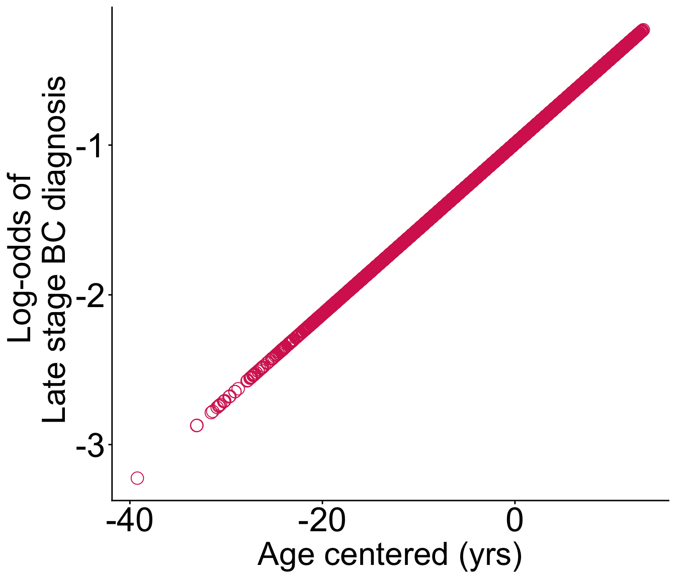
Fitted logistic regression model: \[\text{logit}(\widehat{\pi}(Age)) = -0.989 + 0.057 \cdot Age\]
\(\widehat{\beta}_0\): The estimated log-odds is -0.989 for someone who is 61.71 years (95% CI: -1.035, -0.944)
\(\widehat{\beta}_1\): The estimated increase in log-odds is 0.057 for every 1 year increase in age (95% CI: 0.051, 0.063).
What does a log-odds even mean?? Or an increase in log-odds??
We will need to calculate the odds ratio and its confidence interval
- Then we will visualize the odds ratio

Poll Everywhere Question 1

We typically interpret our results using odds ratios

For our fitted simple logistic regression model with a continuous predictor \[\text{logit}(\widehat{\pi}(X)) = \widehat{\beta}_0 + \widehat{\beta}_1 \cdot X\]

How do we go from interpretations of \(\widehat{\beta}_0\) and \(\widehat{\beta}_1\) using log odds to odds ratios?

We will need to take the exponential of our model:
- \(\text{exp}(\widehat{\beta}_0)\): expected odds that \(Y=1\) when X is 0.
- \(\text{exp}(\widehat{\beta}_1)\): expected odds ratio that \(Y=1\) for every 1 unit increase in X

Important distinction:
- We take the inverse logit to find our predicted probability
- We take the exponential to interpret the odds/odds ratios

Intro/Recap of Interpreting Fitted Model

Interpret coefficients from fitted logistic regression model
- Goodness-of-fit of model should be assessed before summarizing findings (have not covered yet)
- In this lecture: assume model fits data well

The interpretation of the coefficients involves two issues:
- The functional relationship between the dependent variable and the independent variable (link function)
- Unit of change for the independent variable

We will learn the interpretation for
- Binary independent variable
- Categorical independent variable with multiple groups
  - We looked at this for our race and ethnicity variable
- Continuous independent variable

Learning Objectives

Interpret odds ratios from fitted simple logistic regression model for a continuous explanatory variable.

Interpret odds ratios from fitted simple logistic regression model for a binary explanatory variable.
Interpret odds ratios from fitted simple logistic regression model for a multi-level categorical explanatory variable.
Report the odds ratio using a table and/or a forest plot.

Coefficient interpretation: Continuous Independent Variable

For simplicity, we assume the linear relationship between logit and continuous variable \(X\)

Again using simple logistic regression model to illustrate the interpretation of \(\widehat{\beta}\) for a continuous variable \(X\) \[\text{logit}(\widehat{\pi}(X)) = \widehat{\beta}_0 + \widehat{\beta}_1 \cdot X\]

The estimated slope coefficient, \(\widehat{\beta}_1\), is the expected change in the log odds for 1 unit increase in \(X\)
- Additional attention should be paid to picking a meaningful units of change in \(X\)

How do we get the odds ratio for X’s coefficient?

For \(\text{exp}(\widehat{\beta}_1)\)

We compare \(X=x\) and \(X=x+1\),
So we have \[\text{logit}(\widehat{\pi}(X = x)) = \widehat{\beta}_0 + \widehat{\beta}_1 \cdot x\] and \[\text{logit}(\widehat{\pi}(X = x+1)) = \widehat{\beta}_0 + \widehat{\beta}_1 \cdot (x+1)\]
And… \[\begin{aligned} & \text{logit}(\widehat{\pi}(X = x+1)) - \text{logit}(\widehat{\pi}(X = x)) \\ & = \widehat{\beta}_0 + \widehat{\beta}_1 \cdot (x+1) - \big[\widehat{\beta}_0 + \widehat{\beta}_1 \cdot x \big] \\ &= \widehat{\beta}_0 + \widehat{\beta}_1 \cdot x + \widehat{\beta}_1 - \widehat{\beta}_0 - \widehat{\beta}_1 \cdot x \\ & = \widehat{\beta}_1 \end{aligned}\]

Thus, \[\begin{aligned} \widehat{\beta}_1 & = \text{logit}(\widehat{\pi}(X = x+1)) - \text{logit}(\widehat{\pi}(X = x)) \\ \widehat{\beta}_1 & = \text{log}\Bigg(\dfrac{\widehat{\pi}(X=x+1)}{1-\widehat{\pi}(X=x+1)}\Bigg) - \text{log}\Bigg(\dfrac{\widehat{\pi}(X=x)}{1-\widehat{\pi}(X=x)}\Bigg) \\ \widehat{\beta}_1 & = \text{log}\left(\dfrac{\dfrac{\widehat{\pi}(X=x+1)}{1-\widehat{\pi}(X=x+1)}} {\dfrac{\widehat{\pi}(X=x)}{1-\widehat{\pi}(X=x)}}\right) \\ \text{exp}\big[\widehat{\beta}_1\big] & = \text{exp}\left[\text{log}\left(\dfrac{\widehat{\text{odds}}_{X=x+1}} {\widehat{\text{odds}}_{X=x}}\right) \right] \\ \text{exp}\big[\widehat{\beta}_1\big] & = \dfrac{\widehat{\text{odds}}_{X=x+1}} {\widehat{\text{odds}}_{X=x}} \\ \end{aligned}\]

Example: Interpretation of Age Coefficient/OR

In log-odds scale:

\[\widehat{\beta}_1 = 0.057\]

One year increase in age is associated with expected 0.057 increase in log-odds of receiving a late stage breast cancer diagnosis

In odds scale:

\[\exp\left({\widehat{\beta}}_1\right) = 1.06\]

One year increase in age is associated with expected 1.06 times the odds of receiving a late stage breast cancer diagnosis
- Can also say: For every one year increase in age, the expected odds of late stage breast cancer diagnosis increases 1.06 times.
Can also subtract 1 from the odds ratio and multiply by 100 to obtain the percentage change in odds for 1-unit increase.
- 1-year increase in age is associated with an 6% increase in the predicted odds of late stage diagnosis

Example: Age and Late Stage Diagnosis (1/5)

Odds ratio from logistic regression

Compute the estimate and 95% confidence interval for odds ratio for late stage breast cancer diagnosis for every 1 year increase in age.

Needed steps:

Fit the regression model
Transform the coefficients into odds ratios
Interpret the odds ratio

Example: Age and Late Stage Diagnosis (2/5)

Odds ratio from logistic regression

Compute the estimate and 95% confidence interval for odds ratio for late stage breast cancer diagnosis for every 1 year increase in age.

Fit the regression model

bc_reg = bc %>%
  glm(formula = Late_stage_diag ~ Age_c, family = binomial)

Example: Age and Late Stage Diagnosis (3/5)

Odds ratio from logistic regression

Compute the estimate and 95% confidence interval for odds ratio for late stage breast cancer diagnosis for every 1 year increase in age.

Transform the coefficients into odds ratios

Option 1: tidy()

tidy_bc_reg = tidy(bc_reg, conf.int=T, exponentiate = T) 
tidy_bc_reg %>% gt() %>% tab_options(table.font.size = 35) %>%
  fmt_number(decimals = 3)

term	estimate	std.error	statistic	p.value	conf.low	conf.high
(Intercept)	0.372	0.023	−42.637	0.000	0.355	0.389
Age_c	1.059	0.003	17.780	0.000	1.052	1.065

tidy_bc_reg$conf.low # I prefer tidy() bc now I can grab each component

[1] 0.3551931 1.0520321

Example: Age and Late Stage Diagnosis (4/5)

Odds ratio from logistic regression

Compute the estimate and 95% confidence interval for odds ratio for late stage breast cancer diagnosis for every 1 year increase in age.

Transform the coefficients into odds ratios

Option 2: logistic.display()

logistic.display(bc_reg) # Cannot grab each component in this


Logistic regression predicting Late_stage_diag : 1 vs 0 
 
                   OR(95%CI)         P(Wald's test) P(LR-test)
Age_c (cont. var.) 1.06 (1.05,1.07)  < 0.001        < 0.001   
                                                              
Log-likelihood = -5754.8442
No. of observations = 10000
AIC value = 11513.6884

Poll Everywhere Question 2

Example: Age and Late Stage Diagnosis (5/5)

Odds ratio from logistic regression

Compute the estimate and 95% confidence interval for odds ratio for late stage breast cancer diagnosis for every 1 year increase in age.

Interpret the odds ratio

For every one year increase in age, there is an expected 5.86% increase in the odds of late stage breast cancer diagnosis (95% CI: 5.2%, 6.53%).

Transformations of continuous variable to make more interpretable

Sometimes a change in “1” unit may not be considered clinically interesting

For example, a 1 year increase in age or a 1 mm Hg increase in systolic blood pressure may be too small for a meaningful change in log odds
- Instead, we may be interested to find out the log odds change for a increase of 10 years in age or 10 mm Hg in systolic blood pressure

On the other hand, if the range of \(X\) is small (say 0-1), than a change in 1 unit of \(X\) is too large to be meaningful

We should be able to compute and interpret coefficients for a continuous independent covariate \(x\) for an arbitrary change of “c” units in \(x\)

Transformations of continuous variable to make more interpretable

The estimated log odds ratio for a change of c units in x can be obtained from \[\hat{g}\left(x+c\right)-\hat{g}\left(x\right)=c{\hat{\beta}}_1\]
- \(\widehat{OR}\left(c\right)=\exp\left(c{\hat{\beta}}_1\right)\)
The 95% CI for \(\widehat{OR}(c)\) is: \[\exp \left( c \hat{\beta}_1 \pm 1.96 \cdot c \cdot SE_{\hat{\beta}_1} \right)\]
The \(c\) is chosen to be a clinically meaningful unit change in \(x\)
The value of 𝑐 should be clearly specified in all tables and calculations
- Because the estimated OR and the corresponding CI depends on the choice of 𝑐 value

Example: 10 year increase in age and Late Stage Diagnosis

What if we are interested in learning the OR corresponding to 10-year increase in age?

bc_reg = glm(Late_stage_diag ~ Age_c, data = bc, family = binomial)
tidy(bc_reg, conf.int=T) %>% gt() %>% tab_options(table.font.size = 35) %>%
  fmt_number(decimals = 3)

term	estimate	std.error	statistic	p.value	conf.low	conf.high
(Intercept)	−0.989	0.023	−42.637	0.000	−1.035	−0.944
Age_c	0.057	0.003	17.780	0.000	0.051	0.063

Example: 10 year increase in age and Late Stage Diagnosis

What if we are interested in learning the OR corresponding to 10-year increase in age?

\[ \widehat{OR}\left(10\right)=\exp{\left(10\cdot{\hat{\beta}}_1\right)}=\exp{\left(0.56965\right)}=\mathrm{\mathrm{1.767}}\]

The 95% CI for \(\widehat{OR}\left(10\right)\) is: \[\begin{aligned} \widehat{OR}\left(10\right) &=\exp{\left(10\cdot{\hat{\beta}}_1\pm1.96\cdot10\cdot SE_{\hat{\beta}_1} \right)} \\ &=\exp{\left(10\cdot0.056965\pm1.96\cdot10\cdot0.003204\right)}\\ &=(1.66,\ 1.88) \end{aligned}\]

Conclusion: For every 10-year increase in age, the expected odds of late stage breast cancer diagnosis increases 1.77 times (95% CI: 1.66, 1.88).

Example: 10 year increase in age and Late Stage Diagnosis

What if we are interested in learning the OR corresponding to 10-year increase in age?

bc2 = bc %>% mutate(Age_c_10 = Age_c/10)
bc_reg_10 = glm(Late_stage_diag ~ Age_c_10, data = bc2, family = binomial)
tidy(bc_reg_10, conf.int=T, exponentiate = T) %>% gt() %>% tab_options(table.font.size = 35) %>%
  fmt_number(decimals = 3)

term	estimate	std.error	statistic	p.value	conf.low	conf.high
(Intercept)	0.372	0.023	−42.637	0.000	0.355	0.389
Age_c_10	1.768	0.032	17.780	0.000	1.661	1.883

Last Note About Continuous Independent Variable

Notice that the logistic regression model suggests that logit is linear in the covariate
The model implies the additional odds of late stage breast cancer diagnosis for a 40 year-old compared to a 30 year-old is the same as the additional odds of late stage breast cancer diagnosis for a 60 year-old compared to a 50-year-old
This assumption may not be realistic
To address this, we may consider using higher order terms (e.g., \(x^2\), \(x^3\),…) or other nonlinear transformation(e.g., \(log(x)\))
Categorize the continuous variable may be another option
See Lesson 8 and Lesson 14 in our BSTA 512/612 class

How do we get the odds for the intercept?

For \(\text{exp}(\widehat{\beta}_0)\)

When \(X=0\), we have \[\text{logit}(\widehat{\pi}(X=0)) = \widehat{\beta}_0\]
Thus, \[\begin{aligned} \widehat{\beta}_0 & = \text{logit}(\widehat{\pi}(X=0)) \\ \text{exp}\big[\widehat{\beta}_0\big] & = \text{exp}\big[\text{logit}(\widehat{\pi}(X=0))\big] \\ \text{exp}\big[\widehat{\beta}_0\big] & = \text{exp}\Bigg[\text{log}\Bigg(\dfrac{\widehat{\pi}(X=0)}{1-\widehat{\pi}(X=0)}\Bigg)\Bigg] \\ \text{exp}\big[\widehat{\beta}_0\big] & = \dfrac{\widehat{\pi}(X=0)}{1-\widehat{\pi}(X=0)} \\ \end{aligned}\]

Learning Objectives

Interpret odds ratios from fitted simple logistic regression model for a continuous explanatory variable.

Interpret odds ratios from fitted simple logistic regression model for a binary explanatory variable.

Interpret odds ratios from fitted simple logistic regression model for a multi-level categorical explanatory variable.
Report the odds ratio using a table and/or a forest plot.

Coefficient Interpretation: Binary Independent Variable

Independent variable \(X\) is a binary variable (\(X\) can take values: 0 or 1)

We are fitting the population simple logistic regression model: \[\text{logit}\left(\pi(X) \right) = \beta_0 + \beta_1 \cdot I(X=1)\]

The logit difference is \(\beta_1\) for binary independent variable
- \(\beta_1\) represents the change/difference in the logit for \(X=1\) vs. \(X=0\)
  - AKA log odds ratio comparing \(X=1\) to \(X=0\)

It will be much easier to understand if we can interpret the coefficient using odds ratio (OR)

Binary predictor: How do we interpret the coefficient? (1/2)

For individuals with \(X=0\): \[\text{logit}\left(\pi(X=0)\right)=\beta_0+\beta_1\times\left(0\right)=\beta_0\]

For individuals with \(X=1\): \[\text{logit}\left(\pi(X=1)\right)=\beta_0+\beta_1\times\left(1\right)=\beta_0 + \beta_1\]

To solve for \(\beta_1\), we take the difference of the logits: \[ \text{logit}\left(\pi(X=1)\right) - \text{logit}\left(\pi(X=0)\right) = \left( \beta_0 + \beta_1 \right) - \left( \beta_0 \right) = \beta_1\]

Binary predictor: How do we interpret the coefficient? (2/2)

\[ \text{logit}\left(\pi(X=1)\right) - \text{logit}\left(\pi(X=0)\right) = \left( \beta_0 + \beta_1 \right) - \left( \beta_0 \right) = \beta_1\]

\[\begin{aligned} \beta_1&=l\mathrm{ogit}\left(\pi(X=1)\right)\ -l\mathrm{ogit}\left(\pi\left(X=0\right)\right) \\ \beta_1&=l\mathrm{og}\left(\dfrac{\pi(X=1)}{1-\pi(X=1)}\right)-l\mathrm{og}\left(\dfrac{\pi\left(X=0\right)}{1-\pi\left(X=0\right)}\right) \\ \beta_1&=\log{\left(\dfrac{\dfrac{\pi(X=1)}{1-\pi(X=1)}}{\dfrac{\pi(X=0)}{1-\pi(X=0)}}\right)} \\ \exp{\left(\beta_1\right)}&=\dfrac{\dfrac{\pi(X=1)}{1-\pi(X=1)}}{\dfrac{\pi(X=0)}{1-\pi(X=0)}} \end{aligned}\]

Poll Everywhere Question 3

Example: Binary age and Late Stage Diagnosis (1/4)

Odds ratio from logistic regression

What is the odds ratio of late stage breast cancer diagnosis for older individuals (>65 years old) compared to younger individuals (≤65 years old)?

Two options to calculate this value:
- Option 1: Calculate \(\widehat{OR}\) from 2x2 contingency table
  - Try at home: Refer to Lesson 3 for this process
- Option 2: Calculate \(\widehat{OR}\) from logistic regression

Needed steps for Option 2:

Fit the regression model
Transform the coefficients into odds ratios
Interpret the odds ratio

Example: Binary age and Late Stage Diagnosis (2/4)

Odds ratio from logistic regression

What is the odds ratio of late stage breast cancer diagnosis for older individuals (>65 years old) compared to younger individuals (≤65 years old)?

Fit the regression model

bc3 = bc %>% mutate(Age_binary = ifelse(Age > 65, 1, 0))
age_bin_glm = bc3 %>% glm(formula = Late_stage_diag ~ Age_binary, family = binomial)

Example: Binary age and Late Stage Diagnosis (3/4)

Odds ratio from logistic regression

What is the odds ratio of late stage breast cancer diagnosis for older individuals (>65 years old) compared to younger individuals (≤65 years old)?

Transform the coefficients into odds ratios

age_bin_tidy = tidy(age_bin_glm, conf.int=T, exponentiate = T) 
age_bin_tidy %>% gt() %>%
  tab_options(table.font.size = 35) %>%
  fmt_number(decimals = 3)

term	estimate	std.error	statistic	p.value	conf.low	conf.high
(Intercept)	0.297	0.031	−39.608	0.000	0.280	0.315
Age_binary	1.875	0.045	13.928	0.000	1.716	2.048

Poll Everywhere Question 4

Example: Binary age and Late Stage Diagnosis (4/4)

Odds ratio from logistic regression

What is the odds ratio of late stage breast cancer diagnosis for older individuals (>65 years old) compared to younger individuals (≤65 years old)?

Interpret the odds ratio

The estimated odds of late stage breast cancer among individuals over 65 years old is 1.87 (95% CI: (1.72, 2.05)) times that of individuals 65 years or younger.

Learning Objectives

Interpret odds ratios from fitted simple logistic regression model for a continuous explanatory variable.
Interpret odds ratios from fitted simple logistic regression model for a binary explanatory variable.

Interpret odds ratios from fitted simple logistic regression model for a multi-level categorical explanatory variable.

Report the odds ratio using a table and/or a forest plot.

Coefficient Interpretation: Multi-group Categorical Variable

Independent variable \(X\) is a multi-level categorical variable

Let’s say \(X\) takes values: a, b, c, or d

We are fitting the simple logistic regression model: \[\text{logit}\left(\pi(X) \right) = \beta_0 + \beta_1 \cdot I(X=b) + \beta_2 \cdot I(X=c) + \beta_3 \cdot I(X=d)\]
- Where \(a\) is our reference group

\(\beta_1\) represents the change/difference in the log-odds for \(X=b\) vs. \(X=a\)
- AKA log odds ratio comparing \(X=b\) to \(X=a\)

Coefficient Interpretation: Multi-group Categorical Variable

We are fitting the simple logistic regression model with reference group \(a\): \[\text{logit}\left(\pi(X) \right) = \beta_0 + \beta_1 \cdot I(X=b) + \beta_2 \cdot I(X=c) + \beta_3 \cdot I(X=d)\]

\(\beta_0\): the log-odds of event \(Y=1\) for group \(a\)

\(\beta_1\): the difference in log-odds of event \(Y=1\) comparing group \(b\) to group \(a\)

\(\beta_2\): the difference in log-odds of event \(Y=1\) comparing group \(c\) to group \(a\)

\(\beta_3\): the difference in log-odds of event \(Y=1\) comparing group \(d\) to group \(a\)

Multi-level categorical: How do we interpret the coefficient? (II)

\[ \text{logit}\left(\pi(X=c)\right) - \text{logit}\left(\pi(X=a)\right) = \left( \beta_0 + \beta_1\cdot 0 + \beta_2\cdot 1 + \beta_3\cdot 0 \right) - \left( \beta_0 + \beta_1\cdot 0 + \beta_2\cdot 0 + \beta_3\cdot 0 \right) = \beta_2\]

\[\begin{aligned} \beta_2&=l\mathrm{ogit}\left(\pi(X=c)\right)\ -l\mathrm{ogit}\left(\pi\left(X=a\right)\right) \\ \beta_2&=l\mathrm{og}\left(\dfrac{\pi(X=c)}{1-\pi(X=c)}\right)-l\mathrm{og}\left(\dfrac{\pi\left(X=a\right)}{1-\pi\left(X=a\right)}\right) \\ \beta_2&=\log{\left(\dfrac{\dfrac{\pi(X=c)}{1-\pi(X=c)}}{\dfrac{\pi(X=a)}{1-\pi(X=a)}}\right)} \\ \exp{\left(\beta_2\right)}&=\dfrac{\dfrac{\pi(X=c)}{1-\pi(X=c)}}{\dfrac{\pi(X=a)}{1-\pi(X=a)}} \end{aligned}\]

Coefficient Interpretation: Multi-group Categorical Variable

We are fitting the simple logistic regression model with reference group \(a\): \[\text{logit}\left(\pi(X) \right) = \beta_0 + \beta_1 \cdot I(X=b) + \beta_2 \cdot I(X=c) + \beta_3 \cdot I(X=d)\]

\(\exp\left(\beta_0\right)\): the odds of event \(Y=1\) for group \(a\)
\(\exp\left(\beta_1\right)\): the odds of event \(Y=1\) for group \(b\) is \(\exp\left(\beta_1\right)\) times the odds of event \(Y=1\) for group \(a\)
\(\exp\left(\beta_2\right)\): the odds of event \(Y=1\) for group \(c\) is \(\exp\left(\beta_2\right)\) times the odds of event \(Y=1\) for group \(a\)
\(\exp\left(\beta_3\right)\): the odds of event \(Y=1\) for group \(d\) is \(\exp\left(\beta_3\right)\) times the odds of event \(Y=1\) for group \(a\)

Remember, as soon as we fit the regression model, we talk about the “expected odds” or “estimated odds”

How do we pick the reference group?

The choice can be more apparent for multi-group categorical independent variables within studies

For example, if we want to evaluate the association between clinical response and four treatments.
- The treatment variable has 4 categories: “active treatment A”, “active treatment B”, “active treatment C” and “Placebo treatment”
- The investigator is interested in comparing each of the three active treatment with the placebo treatment
- Then the placebo treatment should be picked as the reference group

In this class, we will try our best to pick a reference from our own knowledge…
- but in general this is a decision I make with someone who has expertise in the field of study

Example: Late stage diagnosis and race and ethnicity

We chose Non-Hispanic White individuals as reference group

Underlying health disparities linked to racism in healthcare and in clinical studies

There is evidence that white individuals receive a certain standard of care that is not paralleled for POC (Mateo and Williams (2021))

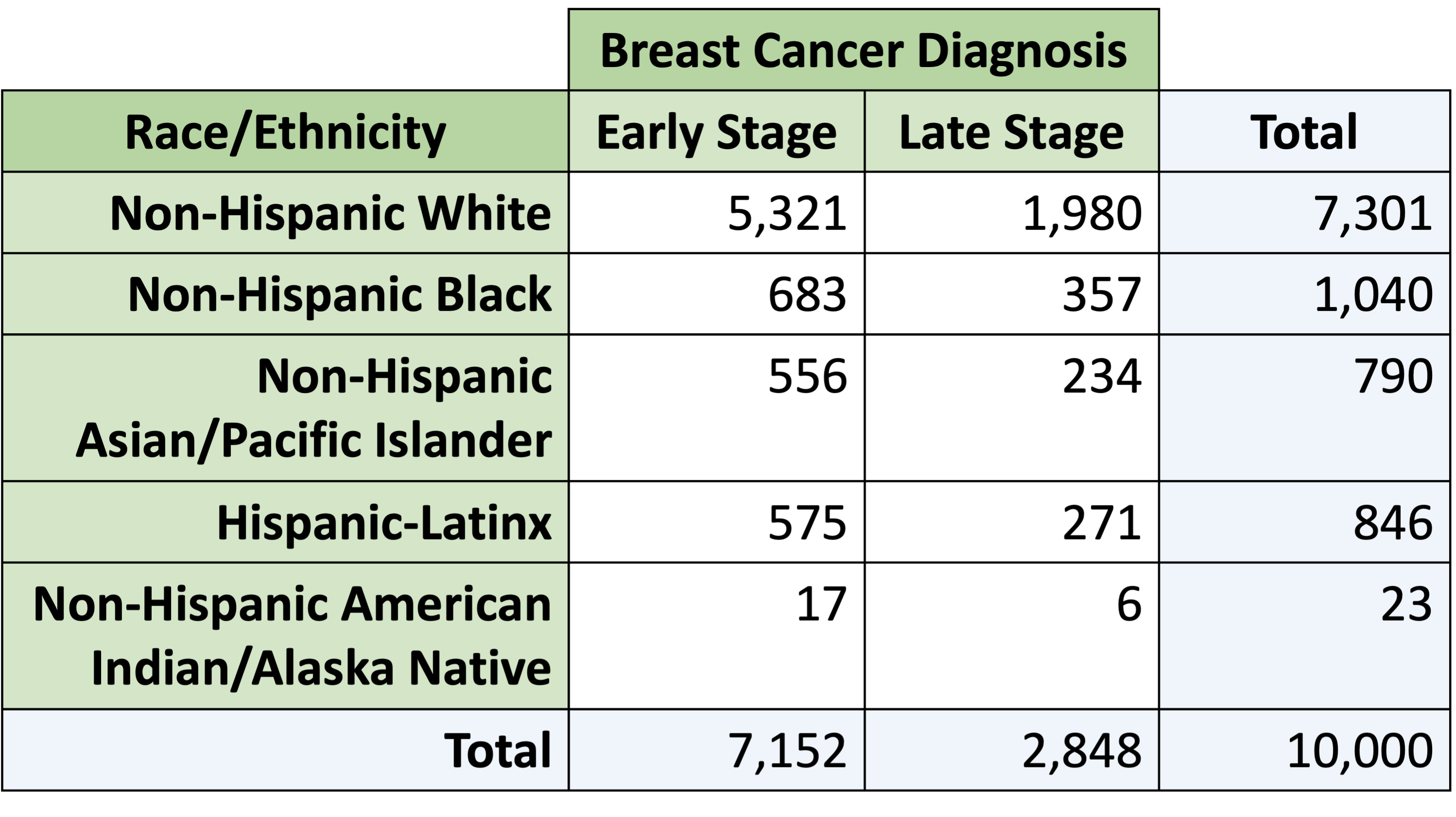
Something else to consider: if your reference group does not have a lot of individuals, then you may not see any statistical significance!

Example: Late stage diagnosis and race and ethnicity

Odds ratio from logistic regression

What is the odds ratio of late stage breast cancer diagnosis for Non-Hispanic Asian/Pacific Islander individuals compared to Non-Hispanic White individuals?

Needed steps:

Fit the regression model
Transform the coefficients into odds ratios
Interpret the odds ratio

Example: Late stage diagnosis and race and ethnicity

Odds ratio from logistic regression

What is the odds ratio of late stage breast cancer diagnosis for Non-Hispanic Asian/Pacific Islander individuals compared to Non-Hispanic White individuals?

Fit the regression model

RE_glm = bc %>% 
  glm(formula = Late_stage_diag ~ Race_Ethnicity, family = binomial)

\[ \begin{aligned} \text{logit}\left(\pi(X) \right) = & \beta_0 + \beta_1 \cdot I(X=\text{Hispanic-Latino}) + \\ & \beta_2 \cdot I(X=\text{NH American Indian/Alaskan Native}) + \\ & \beta_3 \cdot I(X=\text{NH Asian/Pacific Islander}) + \\ & \beta_4 \cdot I(X=\text{NH Black}) \end{aligned} \]

Example: Late stage diagnosis and race and ethnicity

Odds ratio from logistic regression

What is the odds ratio of late stage breast cancer diagnosis for Non-Hispanic Asian/Pacific Islander individuals compared to Non-Hispanic White individuals?

Transform the coefficients into odds ratios

RE_tidy = tidy(RE_glm, conf.int=T, exponentiate = T) 
RE_tidy %>% gt() %>%
  tab_options(table.font.size = 35) %>%
  fmt_number(decimals = 3)

term	estimate	std.error	statistic	p.value	conf.low	conf.high
(Intercept)	0.372	0.026	−37.553	0.000	0.353	0.392
Race_EthnicityHispanic-Latino	0.968	0.082	−0.398	0.691	0.822	1.135
Race_EthnicityNH American Indian/Alaskan Native	0.948	0.476	−0.111	0.911	0.342	2.287
Race_EthnicityNH Asian/Pacific Islander	1.131	0.082	1.497	0.134	0.961	1.327
Race_EthnicityNH Black	1.405	0.070	4.826	0.000	1.223	1.611

Example: Late stage diagnosis and race and ethnicity

Odds ratio from logistic regression

What is the odds ratio of late stage breast cancer diagnosis for Non-Hispanic Asian/Pacific Islander individuals compared to Non-Hispanic White individuals?

Interpret the odds ratio

The estimated odds of late stage breast cancer among Non-Hispanic Asian/Pacific Islander individuals is 1.13 (95% CI: (0.96, 1.33)) times that of Non-Hispanic White individuals.

What if you want to compare other groups?

What if we want to estimate OR comparing Non-Hispanic Asian Pacific Islander to Non-Hispanic Black individuals?
Option 1: Change reference group and refit the model (maybe the easiest option)
Option 2: Estimate OR using fitted coefficients (\(\widehat{\beta}\)’s) in the current model: \[\begin{aligned} \text{log}\left( OR (\text{NH API}, \text{NH B}) \right) &= \text{logit}\left(\pi \left(X = \text{NH API}\right)\right) - \text{logit}\left(\pi \left(X = \text{NH B}\right)\right) \\ & = \left[\beta_0 + \beta_3 \cdot 1\right] - \left[\beta_0 + \beta_4 \cdot 1 \right] \\ \text{log}\left( \widehat{OR} (\text{NH API}, \text{NH B}) \right) &= \widehat{\beta}_3 - \widehat{\beta}_4 \\ \widehat{OR} (\text{NH API}, \text{NH B}) &= \exp \left( \widehat{\beta}_3 - \widehat{\beta}_4 \right) \end{aligned}\]

Reference: Using `estimable()` in Option 2

We could use estimable() to calculate this linear combination of coefficients (see BSTA 512 Lesson)

library(gmodels)
RE_glm %>% estimable(
                   c("(Intercept)"                                     = 0,   # beta0
                     "Race_EthnicityHispanic-Latino"                   = 0,   # beta1
                     "Race_EthnicityNH American Indian/Alaskan Native" = 0,   # beta2
                     "Race_EthnicityNH Asian/Pacific Islander"         = 1,   # beta3
                     "Race_EthnicityNH Black"                          = -1), # beta4
                   conf.int = 0.95) %>% 
  exp(.)

              Estimate Std. Error X^2 value       DF Pr(>|X^2|)  Lower.CI
(0 0 0 1 -1) 0.8051811   1.107021  93.89366 2.718282   1.033623 0.6580966
              Upper.CI
(0 0 0 1 -1) 0.9851389

Poll Everywhere Question 5

What if you want to compare other groups? Option 1

bc3 = bc %>% 
  mutate(Race_Ethnicity = fct_relevel(Race_Ethnicity, "NH Black"))
RE_glm2 = glm(Late_stage_diag ~ Race_Ethnicity, data = bc3, 
               family = binomial)
tidy(RE_glm2, conf.int=T, exponentiate = T) %>% gt() %>%
  tab_options(table.font.size = 38) %>%
  fmt_number(decimals = 3)

term	estimate	std.error	statistic	p.value	conf.low	conf.high
(Intercept)	0.523	0.065	−9.934	0.000	0.459	0.594
Race_EthnicityNH White	0.712	0.070	−4.826	0.000	0.621	0.818
Race_EthnicityHispanic-Latino	0.689	0.102	−3.664	0.000	0.564	0.840
Race_EthnicityNH American Indian/Alaskan Native	0.675	0.479	−0.819	0.413	0.242	1.641
Race_EthnicityNH Asian/Pacific Islander	0.805	0.102	−2.131	0.033	0.659	0.982

Learning Objectives

Interpret odds ratios from fitted simple logistic regression model for a continuous explanatory variable.
Interpret odds ratios from fitted simple logistic regression model for a binary explanatory variable.
Interpret odds ratios from fitted simple logistic regression model for a multi-level categorical explanatory variable.

Report the odds ratio using a table and/or a forest plot.

How to present odds ratios: Table

tbl_regression() in the gtsummary package is helpful for presenting the odds ratios in a clean way

library(gtsummary)
tbl_regression(RE_glm, exponentiate = TRUE) %>% 
  as_gt() %>% # allows us to use tab_options()
  tab_options(table.font.size = 38)

Characteristic	OR	95% CI	p-value
Race_Ethnicity
NH White	—	—
Hispanic-Latino	0.97	0.82, 1.14	0.7
NH American Indian/Alaskan Native	0.95	0.34, 2.29	>0.9
NH Asian/Pacific Islander	1.13	0.96, 1.33	0.13
NH Black	1.40	1.22, 1.61	<0.001
Abbreviations: CI = Confidence Interval, OR = Odds Ratio

How to present odds ratios: Forest Plot Setup

Check out my reference on making a forest plot!

library(broom.helpers)
RE_tidy = tidy_and_attach(RE_glm, conf.int=T, exponentiate = T) %>%
  tidy_remove_intercept() %>%
  tidy_add_reference_rows() %>% tidy_add_estimate_to_reference_rows() %>%
  tidy_add_term_labels()
glimpse(RE_tidy)

Rows: 5
Columns: 16
$ term           <chr> "Race_EthnicityNH White", "Race_EthnicityHispanic-Latin…
$ variable       <chr> "Race_Ethnicity", "Race_Ethnicity", "Race_Ethnicity", "…
$ var_label      <chr> "Race_Ethnicity", "Race_Ethnicity", "Race_Ethnicity", "…
$ var_class      <chr> "factor", "factor", "factor", "factor", "factor"
$ var_type       <chr> "categorical", "categorical", "categorical", "categoric…
$ var_nlevels    <int> 5, 5, 5, 5, 5
$ contrasts      <chr> "contr.treatment", "contr.treatment", "contr.treatment"…
$ contrasts_type <chr> "treatment", "treatment", "treatment", "treatment", "tr…
$ reference_row  <lgl> TRUE, FALSE, FALSE, FALSE, FALSE
$ label          <chr> "NH White", "Hispanic-Latino", "NH American Indian/Alas…
$ estimate       <dbl> 1.0000000, 0.9678002, 0.9484848, 1.1310170, 1.4046741
$ std.error      <dbl> NA, 0.08224948, 0.47558680, 0.08224988, 0.07041472
$ statistic      <dbl> NA, -0.3979312, -0.1112089, 1.4968682, 4.8257715
$ p.value        <dbl> NA, 6.906809e-01, 9.114507e-01, 1.344276e-01, 1.394623e…
$ conf.low       <dbl> NA, 0.8223138, 0.3417844, 0.9612074, 1.2226824
$ conf.high      <dbl> NA, 1.135332, 2.286596, 1.327092, 1.611466

How to present odds ratios: Forest Plot

ggplot(data=RE_tidy, aes(y=label, x=estimate, xmin=conf.low, xmax=conf.high)) + 
  geom_point(size = 3) +  geom_errorbarh(height=.2) + 
  geom_vline(xintercept=1, color='#C2352F', linetype='dashed', alpha=1) +
  theme_classic() +
  labs(x = "Estimated OR (95% CI)", y = "Race and ethnicity", 
       title = "Odds ratios of late stage breast cancer diagnosis") +
  theme(axis.title = element_text(size = 25), axis.text = element_text(size = 25), title = element_text(size = 24))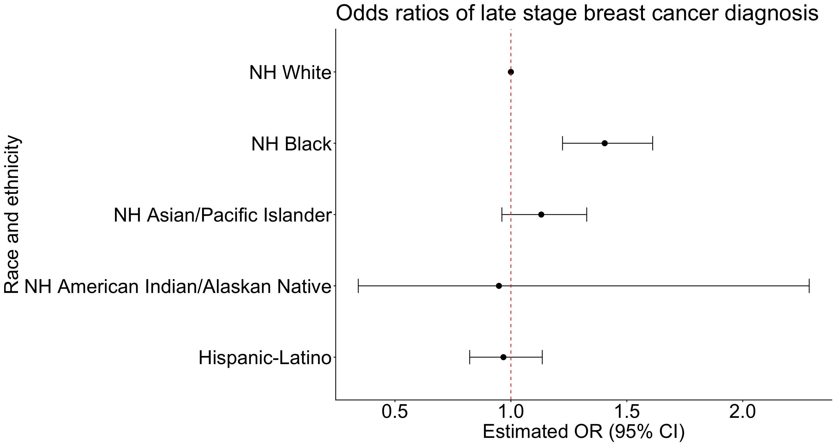

References

Mateo, Camila M., and David R. Williams. 2021. “Racism: A Fundamental Driver of Racial Disparities in Health-Care Quality.” Nature Reviews Disease Primers 7 (1): 1–2. https://doi.org/10.1038/s41572-021-00258-1.

Yedjou, Clement G., Jennifer N. Sims, Lucio Miele, et al. 2019. “Health and Racial Disparity in Breast Cancer.” Advances in Experimental Medicine and Biology 1152: 31–49. https://doi.org/10.1007/978-3-030-20301-6_3.

Lesson 6: Interpretations and Visualizations of Odds Ratios

Learning Objectives

Recall our example: Late stage breast cancer diagnosis

Coefficients on the log-odds scale

Recall our example: Late stage breast cancer diagnosis

Poll Everywhere Question 1

We typically interpret our results using odds ratios

Intro/Recap of Interpreting Fitted Model

Learning Objectives

Coefficient interpretation: Continuous Independent Variable

How do we get the odds ratio for X’s coefficient?

Example: Interpretation of Age Coefficient/OR

Example: Age and Late Stage Diagnosis (1/5)

Example: Age and Late Stage Diagnosis (2/5)

Example: Age and Late Stage Diagnosis (3/5)

Example: Age and Late Stage Diagnosis (4/5)

Poll Everywhere Question 2

Example: Age and Late Stage Diagnosis (5/5)

Transformations of continuous variable to make more interpretable

Transformations of continuous variable to make more interpretable

Example: 10 year increase in age and Late Stage Diagnosis

Example: 10 year increase in age and Late Stage Diagnosis

Example: 10 year increase in age and Late Stage Diagnosis

Last Note About Continuous Independent Variable

How do we get the odds for the intercept?

Learning Objectives

Coefficient Interpretation: Binary Independent Variable

Binary predictor: How do we interpret the coefficient? (1/2)

Binary predictor: How do we interpret the coefficient? (2/2)

Poll Everywhere Question 3

Example: Binary age and Late Stage Diagnosis (1/4)

Example: Binary age and Late Stage Diagnosis (2/4)

Example: Binary age and Late Stage Diagnosis (3/4)

Poll Everywhere Question 4

Example: Binary age and Late Stage Diagnosis (4/4)

Learning Objectives

Coefficient Interpretation: Multi-group Categorical Variable

Coefficient Interpretation: Multi-group Categorical Variable

Multi-level categorical: How do we interpret the coefficient? (II)

Coefficient Interpretation: Multi-group Categorical Variable

How do we pick the reference group?

Example: Late stage diagnosis and race and ethnicity

Example: Late stage diagnosis and race and ethnicity

Example: Late stage diagnosis and race and ethnicity

Example: Late stage diagnosis and race and ethnicity

Example: Late stage diagnosis and race and ethnicity

What if you want to compare other groups?

Reference: Using estimable() in Option 2

Poll Everywhere Question 5

What if you want to compare other groups? Option 1

Learning Objectives

How to present odds ratios: Table

How to present odds ratios: Forest Plot Setup

How to present odds ratios: Forest Plot

References

Reference: Using `estimable()` in Option 2