SLR: More inference + Evaluation
Week 1
Learning Objectives
Identify different sources of variation in an Analysis of Variance (ANOVA) table
Using the F-test, determine if there is enough evidence that population slope \(\beta_1\) is not 0
Calculate and interpret the coefficient of determination
Describe the model assumptions made in linear regression using ordinary least squares
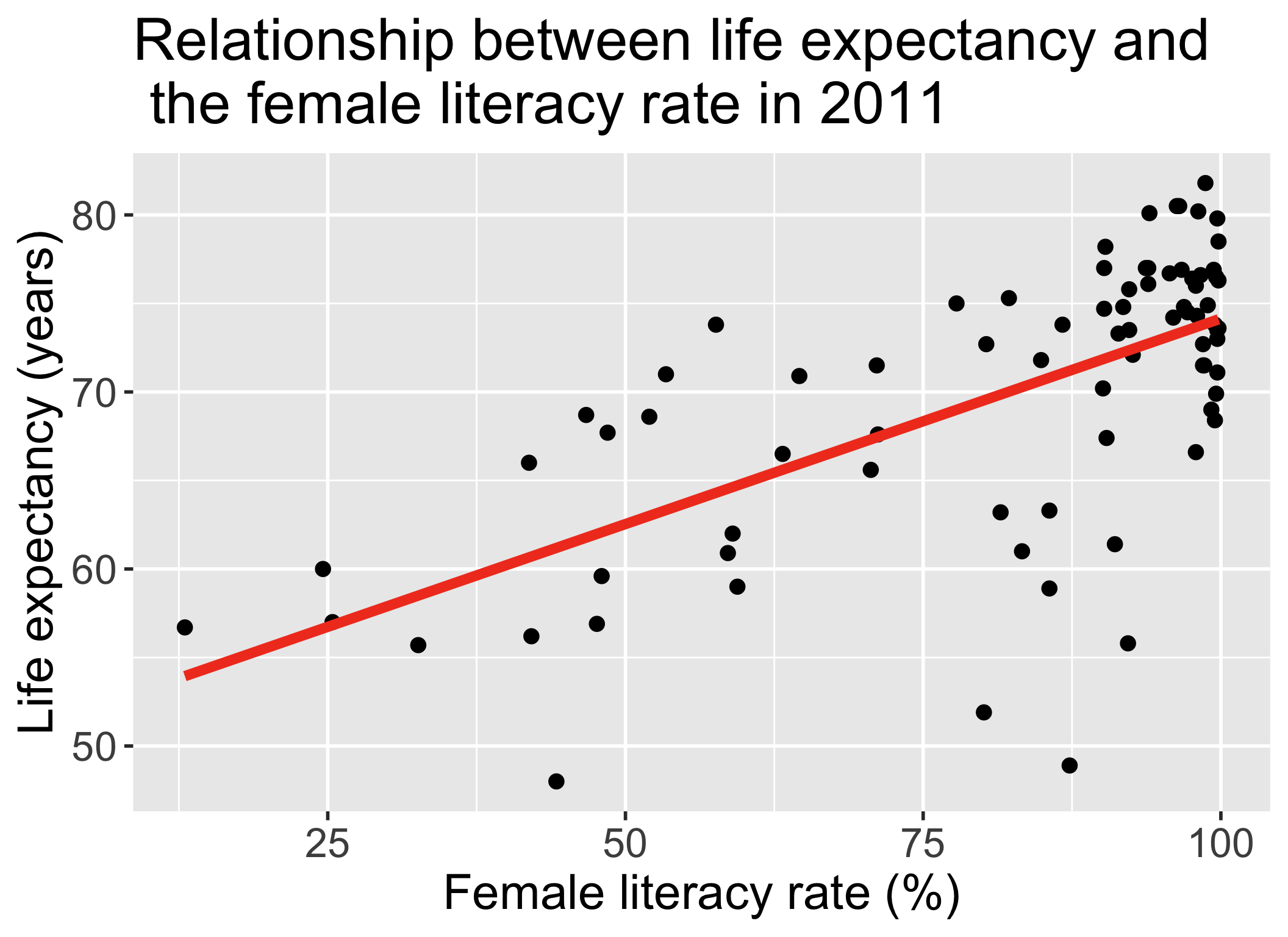
So far in our regression example…
Lesson 1 of SLR:
- Fit regression line
- Calculate slope & intercept
- Interpret slope & intercept
Lesson 2 of SLR:
- Estimate variance of the residuals
- Inference for slope & intercept: CI, p-value
- Confidence bands of regression line for mean value of Y|X
Let’s revisit the regression analysis process

![]()
![]()
Model Selection
Building a model
Selecting variables
Prediction vs interpretation
Comparing potential models
Model Fitting
Find best fit line
Using OLS in this class
Parameter estimation
Categorical covariates
Interactions
Model Evaluation
- Evaluation of model fit
- Testing model assumptions
- Residuals
- Transformations
- Influential points
- Multicollinearity
Model Use (Inference)
- Inference for coefficients
- Hypothesis testing for coefficients
- Inference for expected \(Y\) given \(X\)
- Prediction of new \(Y\) given \(X\)
Learning Objectives
- Identify different sources of variation in an Analysis of Variance (ANOVA) table
Using the F-test, determine if there is enough evidence that population slope \(\beta_1\) is not 0
Calculate and interpret the coefficient of determination
Describe the model assumptions made in linear regression using ordinary least squares
Getting to the F-test
The F statistic in linear regression is essentially a proportion of the variance explained by the model vs. the variance not explained by the model
Start with visual of explained vs. unexplained variation
Figure out the mathematical representations of this variation
Look at the ANOVA table to establish key values measuring our variance from our model
Build the F-test
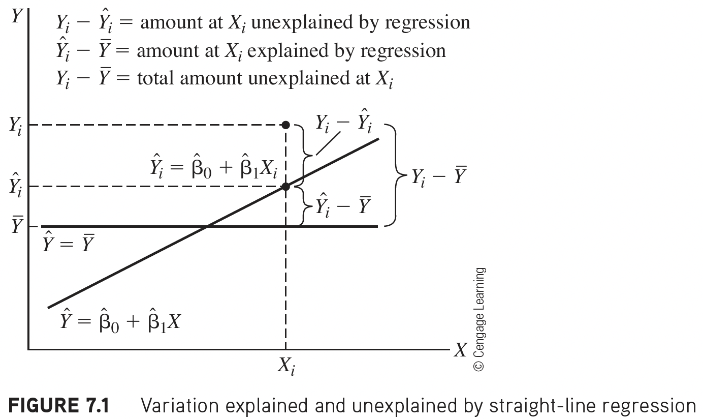
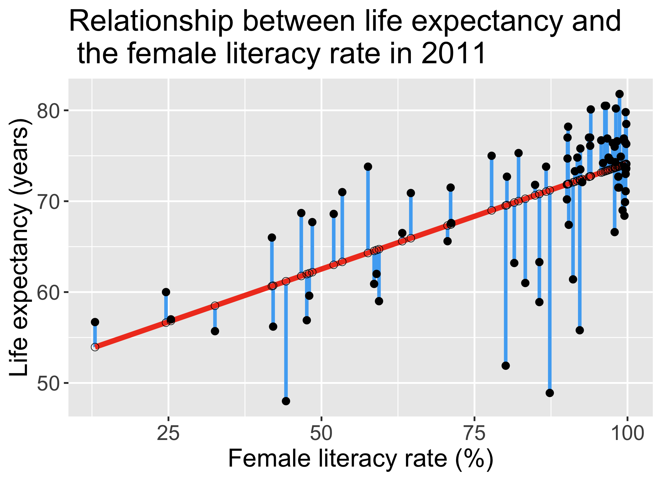
Explained vs. Unexplained Variation
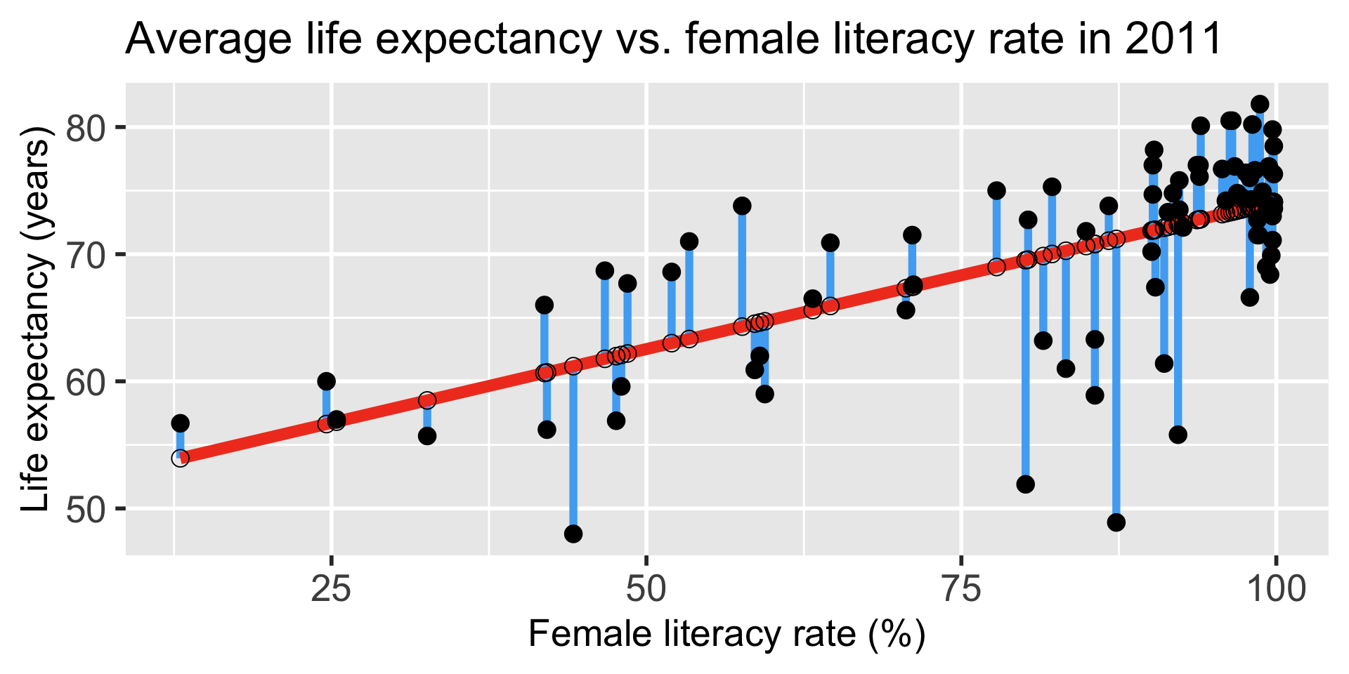
\[ \begin{aligned} Y_i - \overline{Y} & = (Y_i - \hat{Y}_i) + (\hat{Y}_i- \overline{Y})\\ \text{Total unexplained variation} & = \text{Residual variation after regression} + \text{Variation explained by regression} \end{aligned}\]
More on the equation
\[Y_i - \overline{Y} = (Y_i - \hat{Y}_i) + (\hat{Y}_i- \overline{Y})\]
- \(Y_i - \overline{Y}\) = the deviation of \(Y_i\) around the mean \(\overline{Y}\)
- (the total amount deviation unexplained at \(X_i\) ).
- \(Y_i - \hat{Y}_i\) = the deviation of the observation \(Y\) around the fitted regression line
- (the amount deviation unexplained by the regression at \(X_i\) ).
- \(\hat{Y}_i- \overline{Y}\) = the deviation of the fitted value \(\hat{Y}_i\) around the mean \(\overline{Y}\)
- (the amount deviation explained by the regression at \(X_i\) )
Poll Everywhere Question 1
How is this actually calculated for our fitted model?
\[ \begin{aligned} Y_i - \overline{Y} & = (Y_i - \hat{Y}_i) + (\hat{Y}_i- \overline{Y})\\ \text{Total unexplained variation} & = \text{Variation due to regression} + \text{Residual variation after regression} \end{aligned}\]
\[\begin{aligned} \sum_{i=1}^n (Y_i - \overline{Y})^2 & = \sum_{i=1}^n (\hat{Y}_i- \overline{Y})^2 + \sum_{i=1}^n (Y_i - \hat{Y}_i)^2 \\ SSY & = SSR + SSE \end{aligned}\] \[\text{Total Sum of Squares} = \text{Sum of Squares due to Regression} + \text{Sum of Squares due to Error (residuals)}\]
ANOVA table:
| Variation Source | df | SS | MS | test statistic | p-value |
|---|---|---|---|---|---|
| Regression | \(1\) | \(SSR\) | \(MSR = \frac{SSR}{1}\) | \(F = \frac{MSR}{MSE}\) | |
| Error | \(n-2\) | \(SSE\) | \(MSE = \frac{SSE}{n-2}\) | ||
| Total | \(n-1\) | \(SSY\) |
Analysis of Variance (ANOVA) table in R
# Fit regression model:
model1 <- lm(life_expectancy_years_2011 ~ female_literacy_rate_2011,
             data = gapm)

anova(model1)
Analysis of Variance Table
Response: life_expectancy_years_2011
Df Sum Sq Mean Sq F value Pr(>F)
female_literacy_rate_2011 1 2052.8 2052.81 54.414 1.501e-10 ***
Residuals 78 2942.6 37.73
---
Signif. codes: 0 '***' 0.001 '**' 0.01 '*' 0.05 '.' 0.1 ' ' 1anova(model1) %>% tidy() %>% gt() %>%
tab_options(table.font.size = 40) %>%
fmt_number(decimals = 3)| term | df | sumsq | meansq | statistic | p.value |
|---|---|---|---|---|---|
| female_literacy_rate_2011 | 1.000 | 2,052.812 | 2,052.812 | 54.414 | 0.000 |
| Residuals | 78.000 | 2,942.635 | 37.726 | NA | NA |
Learning Objectives
- Identify different sources of variation in an Analysis of Variance (ANOVA) table
- Using the F-test, determine if there is enough evidence that population slope \(\beta_1\) is not 0
Calculate and interpret the coefficient of determination
Describe the model assumptions made in linear regression using ordinary least squares
What is the F statistic testing?
\[F = \frac{MSR}{MSE}\]
- It can be shown that
\[E(MSE)=\sigma^2\ \text{and}\ E(MSR) = \sigma^2 + \beta_1^2\sum_{i=1}^n (X_i- \overline{X})^2\]
- Recall that \(\sigma^2\) is the variance of the residuals
- Thus if
- \(\beta_1 = 0\), then \(F \approx \frac{\hat{\sigma}^2}{\hat{\sigma}^2} = 1\)
- \(\beta_1 \neq 0\), then \(F \approx \frac{\hat{\sigma}^2 + \hat{\beta}_1^2\sum_{i=1}^n (X_i- \overline{X})^2}{\hat{\sigma}^2} > 1\)
- So the \(F\) statistic can also be used to test \(\beta_1\)
F-test vs. t-test for the population slope
The square of a \(t\)-distribution with \(df = \nu\) is an \(F\)-distribution with \(df = 1, \nu\)
\[T_{\nu}^2 \sim F_{1,\nu}\]
- We can use either F-test or t-test to run the following hypothesis test:
- Note that the F-test does not support one-sided alternative tests, but the t-test does!
Planting a seed about the F-test
We can think about the hypothesis test for the slope…
Null \(H_0\)
\(\beta_1=0\)
Alternative \(H_1\)
\(\beta_1\neq0\)
in a slightly different way…
Null model (\(\beta_1=0\))
- \(Y = \beta_0 + \epsilon\)
- Smaller (reduced) model
Alternative model (\(\beta_1\neq0\))
- \(Y = \beta_0 + \beta_1 X + \epsilon\)
- Larger (full) model
In multiple linear regression, we can start using this framework to test multiple coefficient parameters at once
Decide whether or not to reject the smaller reduced model in favor of the larger full model
Cannot do this with the t-test!
Poll Everywhere Question 2
F-test: general steps for hypothesis test for population slope \(\beta_1\)
- For today’s class, we are assuming that we have met the underlying assumptions
- State the null hypothesis.
Often, we are curious if the coefficient is 0 or not:
\[\begin{align} H_0 &: \beta_1 = 0\\ \text{vs. } H_A&: \beta_1 \neq 0 \end{align}\]- Specify the significance level.
Often we use \(\alpha = 0.05\)
- Specify the test statistic and its distribution under the null
The test statistic is \(F\), and follows an F-distribution with numerator \(df=1\) and denominator \(df=n-2\).
- Compute the value of the test statistic
The calculated test statistic for \(\widehat\beta_1\) is
\[F = \frac{MSR}{MSE}\]
- Calculate the p-value
We are generally calculating: \(P(F_{1, n-2} > F)\)
- Write conclusion for hypothesis test
- Reject: \(P(F_{1, n-2} > F) < \alpha\)
We (reject/fail to reject) the null hypothesis that the slope is 0 at the \(100\alpha\%\) significiance level. There is (sufficient/insufficient) evidence that there is significant association between (\(Y\)) and (\(X\)) (p-value = \(P(F_{1, n-2} > F)\)).
Life expectancy example: hypothesis test for population slope \(\beta_1\)
- Steps 1-4 are setting up our hypothesis test: not much change from the general steps
- For today’s class, we are assuming that we have met the underlying assumptions
- State the null hypothesis.
We are testing if the slope is 0 or not:
\[\begin{align} H_0 &: \beta_1 = 0\\ \text{vs. } H_A&: \beta_1 \neq 0 \end{align}\]- Specify the significance level.
Often we use \(\alpha = 0.05\)
- Specify the test statistic and its distribution under the null
The test statistic is \(F\), and follows an F-distribution with numerator \(df=1\) and denominator \(df=n-2 = 80-2\).
nobs(model1)[1] 80Life expectancy example: hypothesis test for population slope \(\beta_1\) (2/4)
- Compute the value of the test statistic
anova(model1) %>% tidy() %>% gt() %>%
tab_options(table.font.size = 40)| term | df | sumsq | meansq | statistic | p.value |
|---|---|---|---|---|---|
| female_literacy_rate_2011 | 1 | 2052.812 | 2052.81234 | 54.4136 | 1.501286e-10 |
| Residuals | 78 | 2942.635 | 37.72609 | NA | NA |
- Option 1: Calculate the test statistic using the values in the ANOVA table
\[F = \frac{MSR}{MSE} = \frac{2052.81}{37.73}=54.414\]
- Option 2: Get the test statistic value (F) from the ANOVA table
I tend to skip this step because I can do it all with step 6
Life expectancy example: hypothesis test for population slope \(\beta_1\) (3/4)
- Calculate the p-value
As per Step 4, test statistic \(F\) can be modeled by a \(F\)-distribution with \(df1 = 1\) and \(df2 = n-2\).
- We had 80 countries’ data, so \(n=80\)
Option 1: Use
pf()and our calculated test statistic
# p-value is ALWAYS the right tail for F-test
pf(54.414, df1 = 1, df2 = 78, lower.tail = FALSE)
[1] 1.501104e-10- Option 2: Use the ANOVA table
anova(model1) %>% tidy() %>% gt() %>%
tab_options(table.font.size = 40)| term | df | sumsq | meansq | statistic | p.value |
|---|---|---|---|---|---|
| female_literacy_rate_2011 | 1 | 2052.812 | 2052.81234 | 54.4136 | 1.501286e-10 |
| Residuals | 78 | 2942.635 | 37.72609 | NA | NA |
Life expectancy example: hypothesis test for population slope \(\beta_1\) (4/4)
- Write conclusion for the hypothesis test
We reject the null hypothesis that the slope is 0 at the \(5\%\) significance level. There is sufficient evidence that there is significant association between female life expectancy and female literacy rates (p-value < 0.0001).
Did you notice anything about the p-value?
The p-value of the t-test and F-test are the same!!
- For the t-test:
tidy(model1) %>% gt() %>%
tab_options(table.font.size = 40)| term | estimate | std.error | statistic | p.value |
|---|---|---|---|---|
| (Intercept) | 50.9278981 | 2.66040695 | 19.142898 | 3.325312e-31 |
| female_literacy_rate_2011 | 0.2321951 | 0.03147744 | 7.376557 | 1.501286e-10 |
- For the F-test:
anova(model1) %>% tidy() %>% gt() %>%
tab_options(table.font.size = 40)| term | df | sumsq | meansq | statistic | p.value |
|---|---|---|---|---|---|
| female_literacy_rate_2011 | 1 | 2052.812 | 2052.81234 | 54.4136 | 1.501286e-10 |
| Residuals | 78 | 2942.635 | 37.72609 | NA | NA |
This is true when we use the F-test for a single coefficient!
Learning Objectives
Identify different sources of variation in an Analysis of Variance (ANOVA) table
Using the F-test, determine if there is enough evidence that population slope \(\beta_1\) is not 0
- Calculate and interpret the coefficient of determination
- Describe the model assumptions made in linear regression using ordinary least squares
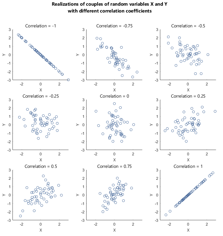
Correlation coefficient from 511
Correlation coefficient \(r\) can tell us about the strength of a relationship
If \(r = -1\), then there is a perfect negative linear relationship between \(X\) and \(Y\)
If \(r = 1\), then there is a perfect positive linear relationship between \(X\) and \(Y\)
If \(r = 0\), then there is no linear relationship between \(X\) and \(Y\)
Note: All other values of \(r\) tell us that the relationship between \(X\) and \(Y\) is not perfect. The closer \(r\) is to 0, the weaker the linear relationship.
Correlation coefficient
The (Pearson) correlation coefficient \(r\) of variables \(X\) and \(Y\) can be computed using the formula:
\[\begin{aligned} r & = \frac{\sum_{i=1}^n (X_i - \overline{X})(Y_i - \overline{Y})}{\Big(\sum_{i=1}^n (X_i - \overline{X})^2 \sum_{i=1}^n (Y_i - \overline{Y})^2\Big)^{1/2}} \\ & = \frac{SSXY}{\sqrt{SSX \cdot SSY}} \end{aligned}\]
we have the relationship
\[\widehat{\beta}_1 = r\frac{SSY}{SSX},\ \ \text{or},\ \ r = \widehat{\beta}_1\frac{SSX}{SSY}\]

Coefficient of determination: \(R^2\)
It can be shown that the square of the correlation coefficient \(r\) is equal to
\[R^2 = \frac{SSR}{SSY} = \frac{SSY - SSE}{SSY}\]
- \(R^2\) is called the coefficient of determination.
- Interpretation: The proportion of variation in the \(Y\) values explained by the regression model
- \(R^2\) measures the strength of the linear relationship between \(X\) and \(Y\):
- \(R^2 = \pm 1\): Perfect relationship
- Happens when \(SSE = 0\), i.e. no error, all points on the line
- \(R^2 = 0\): No relationship
- Happens when \(SSY = SSE\), i.e. using the line doesn’t not improve model fit over using \(\overline{Y}\) to model the \(Y\) values.
- \(R^2 = \pm 1\): Perfect relationship
Poll Everywhere Question
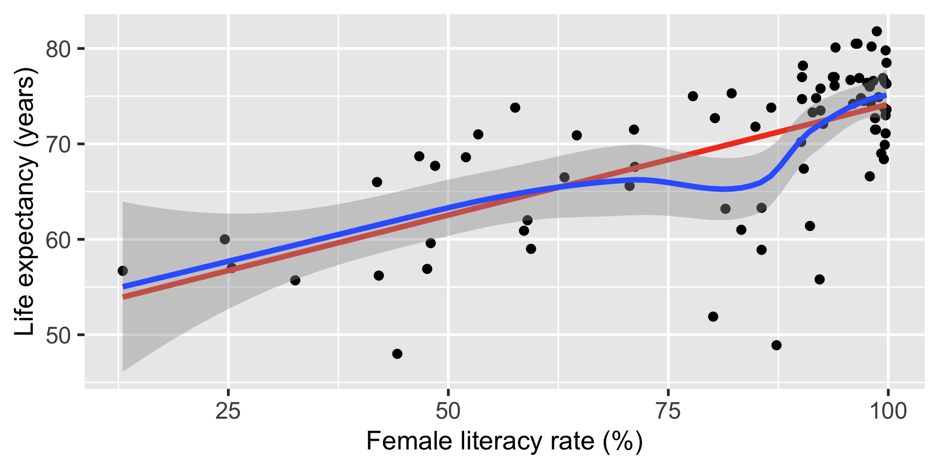
Life expectancy example: correlation coeffiicent \(r\) and coefficient of determination \(R^2\)
(r = cor(x = gapm$life_expectancy_years_2011,
    y = gapm$female_literacy_rate_2011,
    use =  "complete.obs"))
[1] 0.6410434r^2[1] 0.4109366(sum_m1 = summary(model1)) # for R^2 value
Call:
lm(formula = life_expectancy_years_2011 ~ female_literacy_rate_2011,
    data = gapm)

Residuals:
    Min      1Q  Median      3Q     Max
-22.299  -2.670   1.145   4.114   9.498

Coefficients:
                          Estimate Std. Error t value Pr(>|t|)
(Intercept)               50.92790    2.66041  19.143  < 2e-16 ***
female_literacy_rate_2011  0.23220    0.03148   7.377  1.5e-10 ***
---
Signif. codes:  0 '***' 0.001 '**' 0.01 '*' 0.05 '.' 0.1 ' ' 1

Residual standard error: 6.142 on 78 degrees of freedom
Multiple R-squared:  0.4109,    Adjusted R-squared:  0.4034
F-statistic: 54.41 on 1 and 78 DF, p-value: 1.501e-10sum_m1$r.squared[1] 0.4109366
Interpretation
41.1% of the variation in countries’ average life expectancy is explained by the linear model with female literacy rate as the independent variable.
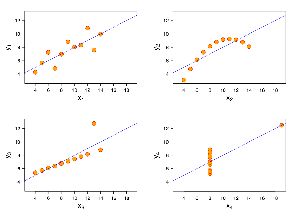
What does \(R^2\) not measure?
\(R^2\) is not a measure of the magnitude of the slope of the regression line
- Example: can have \(R^2 = 1\) for many different slopes!!
\(R^2\) is not a measure of the appropriateness of the straight-line model
- Example: figure
Learning Objectives
Identify different sources of variation in an Analysis of Variance (ANOVA) table
Using the F-test, determine if there is enough evidence that population slope \(\beta_1\) is not 0
Calculate and interpret the coefficient of determination
- Describe the model assumptions made in linear regression using ordinary least squares
Least-squares model assumptions: eLINE
These are the model assumptions made in ordinary least squares:
- e xistence: For any \(X\), there exists a distribution for \(Y\)
- L inearity of relationship between variables
- I ndependence of the \(Y\) values
- N ormality of the \(Y\)’s given \(X\) (residuals)
- E quality of variance of the residuals (homoscedasticity)
e: Existence of Y’s distribution
- For any fixed value of the variable \(X\), \(Y\) is a
- random variable with a certain probability distribution
- having finite
- mean and
- variance
- This leads to the normality assumption
- Note: This is not about \(Y\) alone, but \(Y|X\)
L: Linearity
- The relationship between the variables is linear (a straight line):
- The mean value of \(Y\) given \(X\), \(\mu_{y|x}\) or \(E[Y|X]\), is a straight-line function of \(X\)
\[\mu_{y|x} = \beta_0 + \beta_1 \cdot X\]
I: Independence of observations
- The \(Y\)-values are statistically independent of one another
Examples of when they are not independent, include
- repeated measures (such as baseline, 3 months, 6 months)
- data from clusters, such as different hospitals or families
- This condition is checked by reviewing the study design and not by inspecting the data
- How to analyze data using regression models when the \(Y\)-values are not independent is covered in BSTA 519 (Longitudinal data)
Poll Everywhere Question
N: Normality
- For any fixed value of \(X\), \(Y\) has normal distribution.
- Note: This is not about \(Y\) alone, but \(Y|X\)
- Equivalently, the measurement (random) errors \(\epsilon_i\) ’s normally distributed
- This is more often what we check
- We will discuss how to assess this in practice in Chapter 14 (Regression Diagnostics)
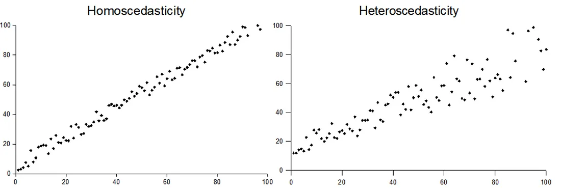
E: Equality of variance of the residuals
The variance of \(Y\) given \(X\) (\(\sigma_{Y|X}^2\)), is the same for any \(X\)
- We use just \(\sigma^2\) to denote the common variance
This is also called homoscedasticity
We will discuss how to assess this in practice in Chapter 14 (Regression Diagnostics)
Summary of eLINE model assumptions
- \(Y\) values are independent (check study design!)
- The distribution of \(Y\) given \(X\) is
- normal
- with mean \(\mu_{y|x} = \beta_0 + \beta_1 \cdot X\)
- and common variance \(\sigma^2\)
- This means that the residuals are
- normal
- with mean = 0
- and common variance \(\sigma^2\)
Anscombe’s Quartet