Missing Data

library(here)
library(tidyverse)
library(mice)
library(naniar)
library(gtsummary)

load(here("project", "data", "wbns_data.rda"))

My variables:

• Outcome: food insecurity

• Predictors:

  • PPAGE: Age
  • LGBT: Gay or lesbian, bisexual, or transgender (re-coded)
  • XACSNET: Internet access
  • PARTNER: Living with a partner
  • FAMSIZE: Family size - field data and imputed
  • INSURED: Insured at time of survey
  • UNMETCARE_Y: Needed medical care but did not get it because could not afford it in past 12 months
  • PPP20197: Citizen
  • PPINCIMP: Household income
  • PPETHM: Race/ethnicity

You should only need to replace my dataset name with yours and my use of variable names with your project’s variables.

There are two blank sections that I invite you to try to complete. These are both important parts of quality assurance. It’s good to check that the distribution of fully observed variables are not different in the missing vs. observed groups of our variables with missing data. Also, it is important to see how our imputed data look if we place it back with the observed data. Do they stand out? I hope not! (I was going to provide code for this, but it’s not new stuff. You can visualize these! … And I really ran out of time this week :( )

Citizenship had missing data that was not coded as NA

I’m using the replace_with_na function to change the missing category to NA.

summary(wbns)

      ID            FOOD_INSEC      PPAGE         LGBT      XACSNET   
 Length:8142        No  :6015   Min.   :18.00   No  :6852   No : 378  
 Class :character   Yes :2069   1st Qu.:36.00   Yes : 621   Yes:7764  
 Mode  :character   NA's:  58   Median :47.00   NA's: 669             
                                Mean   :45.92                         
                                3rd Qu.:57.00                         
                                Max.   :64.00                         
                                                                      
 PARTNER       FAMSIZE     INSURED     UNMETCARE_Y      PPP20197   
 No :7326   2      :3009   No  : 856   No :6725    Yes      :6825  
 Yes: 816   1      :2753   Yes :7167   Yes:1417    Missing  :   5  
            3      : 986   NA's: 119               No       : 470  
            4      : 880                           Not asked: 842  
            5      : 336                                           
            6      : 114                                           
            (Other):  64                                           
                 PPINCIMP                       PPETHM    
 Less than $5,000    : 717   White, Non-Hispanic   :4738  
 $100,000 to $124,999: 641   2+ Races, Non-Hispanic: 238  
 $15,000 to $19,999  : 511   Black, Non-Hispanic   :1023  
 $20,000 to $24,999  : 499   Hispanic              :1473  
 $60,000 to $74,999  : 443   Other, Non-Hispanic   : 670  
 $150,000 to $174,999: 423                                
 (Other)             :4908                                
                        PPEDUCAT   
 Less than high school      : 613  
 Bachelor's degree or higher:3041  
 High school                :1940  
 Some college               :2548  
                                   
                                   
                                   

wbns_miss = wbns %>% 
  replace_with_na(replace = list(PPP20197 = "Missing"))
  # If Missing, replace with NA, if not then keep value as is

summary(wbns_miss)

      ID            FOOD_INSEC      PPAGE         LGBT      XACSNET   
 Length:8142        No  :6015   Min.   :18.00   No  :6852   No : 378  
 Class :character   Yes :2069   1st Qu.:36.00   Yes : 621   Yes:7764  
 Mode  :character   NA's:  58   Median :47.00   NA's: 669             
                                Mean   :45.92                         
                                3rd Qu.:57.00                         
                                Max.   :64.00                         
                                                                      
 PARTNER       FAMSIZE     INSURED     UNMETCARE_Y      PPP20197   
 No :7326   2      :3009   No  : 856   No :6725    Yes      :6825  
 Yes: 816   1      :2753   Yes :7167   Yes:1417    Missing  :   0  
            3      : 986   NA's: 119               No       : 470  
            4      : 880                           Not asked: 842  
            5      : 336                           NA's     :   5  
            6      : 114                                           
            (Other):  64                                           
                 PPINCIMP                       PPETHM    
 Less than $5,000    : 717   White, Non-Hispanic   :4738  
 $100,000 to $124,999: 641   2+ Races, Non-Hispanic: 238  
 $15,000 to $19,999  : 511   Black, Non-Hispanic   :1023  
 $20,000 to $24,999  : 499   Hispanic              :1473  
 $60,000 to $74,999  : 443   Other, Non-Hispanic   : 670  
 $150,000 to $174,999: 423                                
 (Other)             :4908                                
                        PPEDUCAT   
 Less than high school      : 613  
 Bachelor's degree or higher:3041  
 High school                :1940  
 Some college               :2548  
                                   
                                   
                                   

Look at the missing data pattern

Now I can look at the missing data pattern.

md.pattern(wbns_miss, rotate.names = T)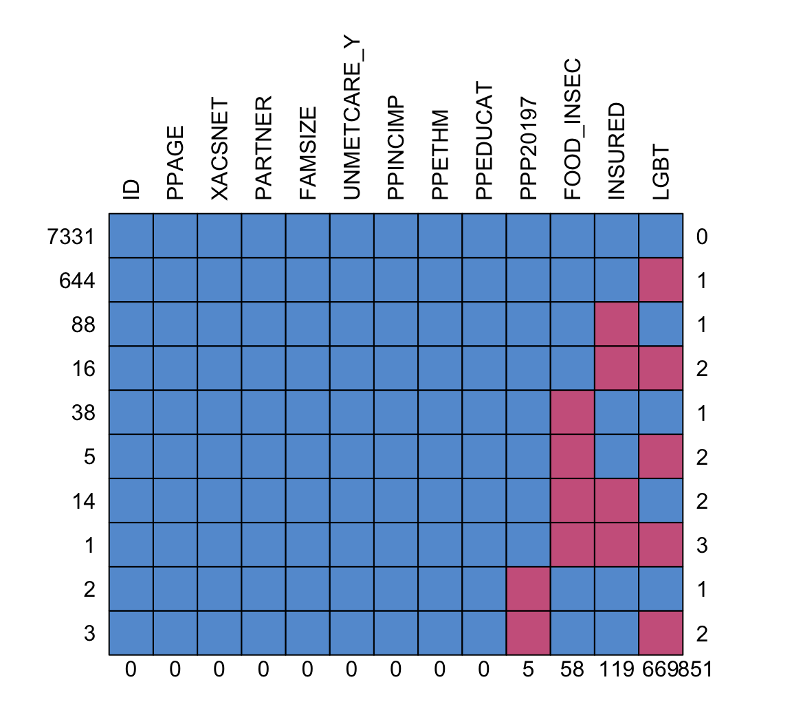

     ID PPAGE XACSNET PARTNER FAMSIZE UNMETCARE_Y PPINCIMP PPETHM PPEDUCAT
7331  1     1       1       1       1           1        1      1        1
644   1     1       1       1       1           1        1      1        1
88    1     1       1       1       1           1        1      1        1
16    1     1       1       1       1           1        1      1        1
38    1     1       1       1       1           1        1      1        1
5     1     1       1       1       1           1        1      1        1
14    1     1       1       1       1           1        1      1        1
1     1     1       1       1       1           1        1      1        1
2     1     1       1       1       1           1        1      1        1
3     1     1       1       1       1           1        1      1        1
      0     0       0       0       0           0        0      0        0
     PPP20197 FOOD_INSEC INSURED LGBT    
7331        1          1       1    1   0
644         1          1       1    0   1
88          1          1       0    1   1
16          1          1       0    0   2
38          1          0       1    1   1
5           1          0       1    0   2
14          1          0       0    1   2
1           1          0       0    0   3
2           0          1       1    1   1
3           0          1       1    0   2
            5         58     119  669 851

Looks like citizenship, food insecurity, insurance, and identifying as LGBT have missing data.

Check the distributions of the variables from the observed vs. missing data

Use mice to impute data

Now we can use the mice() function to impute the data.

Let’s break down what I’m using in the function below:

• I set m=5 as the number of imputations that I will be running

• I set print = F so I don’t get the message as it imputes

• I set defaultMethod = c("norm", "logreg", "polyreg", "polr")

  • This means mice will determine which method to use based on the type of variable
  • For binary variables it will use “logreg.” Thus, it will use logistic regression to predict the missing values. This will include food insecurity, insured, and LGBT variables in my data.
  • For continuous variables, it will use “norm.predict” which will consist of predicting the missing values from linear regression. I don’t have any missing continuous values, so this one is not used.
  • For multi-level categorical varaibles, we use “polyreg” which is a type of logistic regression that is expanded to handle multiple levels of outcomes. This will include citizenship in my data.
  • For ordinal variables, we use “polr” which is a proportional odds model, another type of generalized linear regression model that handles ordered categories. I don’t have any missing ordinal variables, so this one is not used.

wbns_MI_5 = mice(wbns_miss, m=5, print = F, 
                 defaultMethod = c("norm.predict", "logreg", "polyreg", "polr"))

Warning: Number of logged events: 76

Complete data

It’s hard to parse through the output of mice, but we can take a look at one of the imputation’s complete (aka filled in) data. Below I will look at the first imputation (hence the 1). You can change the 1 to anything up to 5 to see the different imputations.

d1 = complete(wbns_MI_5, 1)
summary(d1)

      ID            FOOD_INSEC     PPAGE        LGBT      XACSNET    PARTNER   
 Length:8142        No :6049   Min.   :18.00   No :7455   No : 378   No :7326  
 Class :character   Yes:2093   1st Qu.:36.00   Yes: 687   Yes:7764   Yes: 816  
 Mode  :character              Median :47.00                                   
                               Mean   :45.92                                   
                               3rd Qu.:57.00                                   
                               Max.   :64.00                                   
                                                                               
    FAMSIZE     INSURED    UNMETCARE_Y      PPP20197   
 2      :3009   No : 877   No :6725    Yes      :6827  
 1      :2753   Yes:7265   Yes:1417    Missing  :   0  
 3      : 986                          No       : 472  
 4      : 880                          Not asked: 843  
 5      : 336                                          
 6      : 114                                          
 (Other):  64                                          
                 PPINCIMP                       PPETHM    
 Less than $5,000    : 717   White, Non-Hispanic   :4738  
 $100,000 to $124,999: 641   2+ Races, Non-Hispanic: 238  
 $15,000 to $19,999  : 511   Black, Non-Hispanic   :1023  
 $20,000 to $24,999  : 499   Hispanic              :1473  
 $60,000 to $74,999  : 443   Other, Non-Hispanic   : 670  
 $150,000 to $174,999: 423                                
 (Other)             :4908                                
                        PPEDUCAT   
 Less than high school      : 613  
 Bachelor's degree or higher:3041  
 High school                :1940  
 Some college               :2548  
                                   
                                   
                                   

See how the imputed values look within the observed values

Fit regression with imputations

Below is how we run a regression model with the output from mice (wbns_MI_5). We use the with function that can be read as: With wbns_MI_5, run the following glm function. It will automatically know to know 5 different regressions, one with each imputed dataset.

reg = with(wbns_MI_5, glm(FOOD_INSEC ~ PPAGE + LGBT + XACSNET + PARTNER + 
                                   FAMSIZE + INSURED + UNMETCARE_Y + PPP20197 +
                            PPETHM, family = binomial))

Once I have fit the regression model with each imputed dataset, I can pool the results. The mice function will use Rubin’s Rules to pool the estimates and variances. Note the use of the pool function!

pooled_reg_MI = pool(reg)
mi_reg = summary(pooled_reg_MI, conf.int = TRUE)
mi_reg

                           term    estimate   std.error  statistic        df
1                   (Intercept) -0.94092399 0.191125980 -4.9230565  371.1422
2                         PPAGE  0.00433198 0.002352706  1.8412753 4257.8618
3                       LGBTYes  0.29504789 0.094069406  3.1364915 7823.2657
4                    XACSNETYes -0.53596317 0.120983545 -4.4300502 2633.9023
5                    PARTNERYes  0.74171351 0.091820246  8.0778864 7755.2850
6                      FAMSIZE2 -0.66386257 0.071469877 -9.2887045 7184.0725
7                      FAMSIZE3 -0.30985352 0.093877706 -3.3006082 8042.7947
8                      FAMSIZE4 -0.37783269 0.100154973 -3.7724806 8113.8532
9                      FAMSIZE5 -0.09145848 0.140895783 -0.6491215 7209.2753
10                     FAMSIZE6 -0.13370972 0.233548879 -0.5725128 8115.1279
11                     FAMSIZE7 -0.17014962 0.383547409 -0.4436208 8119.0239
12             FAMSIZE8 or more  0.71359901 0.454899462  1.5686961 8117.4492
13                   INSUREDYes -0.26630423 0.090125051 -2.9548303  267.5774
14               UNMETCARE_YYes  1.63076485 0.065345023 24.9562213 6570.3110
15                   PPP20197No  0.16420384 0.126611682  1.2969091 2663.4593
16            PPP20197Not asked  0.64393756 0.084100957  7.6567210 5487.8370
17 PPETHM2+ Races, Non-Hispanic  0.62960454 0.150679742  4.1784286 8107.6586
18    PPETHMBlack, Non-Hispanic  0.48429429 0.082295957  5.8847884 6012.6999
19               PPETHMHispanic  0.57000522 0.076440622  7.4568365 6839.4712
20    PPETHMOther, Non-Hispanic -0.53485283 0.129266329 -4.1376036 6390.7763
         p.value         2.5 %      97.5 %
1   1.284335e-06 -1.3167495965 -0.56509839
2   6.565074e-02 -0.0002805507  0.00894451
3   1.716164e-03  0.1106467165  0.47944907
4   9.805811e-06 -0.7731955792 -0.29873077
5   7.585129e-16  0.5617210473  0.92170598
6   2.031468e-20 -0.8039645609 -0.52376058
7   9.689561e-04 -0.4938781410 -0.12582891
8   1.627826e-04 -0.5741621197 -0.18150327
9   5.162805e-01 -0.3676555070  0.18473855
10  5.669905e-01 -0.5915253974  0.32410595
11  6.573286e-01 -0.9220008165  0.58170157
12  1.167577e-01 -0.1781205135  1.60531853
13  3.406969e-03 -0.4437486779 -0.08885979
14 2.056988e-131  1.5026673651  1.75886234
15  1.947748e-01 -0.0840633202  0.41247099
16  2.240009e-14  0.4790663555  0.80880877
17  2.966107e-05  0.3342335827  0.92497551
18  4.200523e-09  0.3229647002  0.64562387
19  9.956707e-14  0.4201578390  0.71985261
20  3.554574e-05 -0.7882581666 -0.28144748

We can do an informal sensitivity analysis

Here I am simply running a logistic regression model using our complete data. We can compare the estimates from this model to the pooled estimates from the multiply imputed datasets.

wbns_cc = wbns_miss %>% drop_na()
reg_cc = glm(FOOD_INSEC ~ PPAGE + LGBT + XACSNET + PARTNER + 
               FAMSIZE + INSURED + UNMETCARE_Y + PPP20197 + 
               PPETHM, family = binomial, data = wbns_cc)

cc_reg = summary(reg_cc)

I will put the estimates side-by-side now.

estimates = cbind(Mult_imp = mi_reg$estimate, 
              Complete_case = cc_reg$coefficients[,1])
estimates

                                Mult_imp Complete_case
(Intercept)                  -0.94092399  -0.923507128
PPAGE                         0.00433198   0.003963706
LGBTYes                       0.29504789   0.253429229
XACSNETYes                   -0.53596317  -0.537266195
PARTNERYes                    0.74171351   0.756557601
FAMSIZE2                     -0.66386257  -0.733347778
FAMSIZE3                     -0.30985352  -0.431279163
FAMSIZE4                     -0.37783269  -0.469643349
FAMSIZE5                     -0.09145848  -0.136786735
FAMSIZE6                     -0.13370972  -0.333273866
FAMSIZE7                     -0.17014962  -0.158287657
FAMSIZE8 or more              0.71359901   0.698218128
INSUREDYes                   -0.26630423  -0.242185879
UNMETCARE_YYes                1.63076485   1.739880532
PPP20197No                    0.16420384   0.239127321
PPP20197Not asked             0.64393756   0.596022881
PPETHM2+ Races, Non-Hispanic  0.62960454   0.641231577
PPETHMBlack, Non-Hispanic     0.48429429   0.457402801
PPETHMHispanic                0.57000522   0.535396844
PPETHMOther, Non-Hispanic    -0.53485283  -0.541533105

The most important thing I am noting is that:

1. The complete case estimates have the same signs as the pooled.
2. For the most part, the magnitude of the estimates have not changed by much. Family size seems to be the most impacted.

Now we can proceed with the other parts of Lab 3

Below is some sample code for how I would make a tidy dataset or an odds ratio table from the pooled results! From reg and pooled_reg_MI you should be able to do everything else in Lab 3!

tidy(pooled_reg_MI, exponentiate=T)

                           term  estimate   std.error  statistic       p.value
1                   (Intercept) 0.3902671 0.191125980 -4.9230565  1.284335e-06
2                         PPAGE 1.0043414 0.002352706  1.8412753  6.565074e-02
3                       LGBTYes 1.3431907 0.094069406  3.1364915  1.716164e-03
4                    XACSNETYes 0.5851055 0.120983545 -4.4300502  9.805811e-06
5                    PARTNERYes 2.0995300 0.091820246  8.0778864  7.585129e-16
6                      FAMSIZE2 0.5148588 0.071469877 -9.2887045  2.031468e-20
7                      FAMSIZE3 0.7335544 0.093877706 -3.3006082  9.689561e-04
8                      FAMSIZE4 0.6853452 0.100154973 -3.7724806  1.627826e-04
9                      FAMSIZE5 0.9125992 0.140895783 -0.6491215  5.162805e-01
10                     FAMSIZE6 0.8748440 0.233548879 -0.5725128  5.669905e-01
11                     FAMSIZE7 0.8435386 0.383547409 -0.4436208  6.573286e-01
12             FAMSIZE8 or more 2.0413248 0.454899462  1.5686961  1.167577e-01
13                   INSUREDYes 0.7662060 0.090125051 -2.9548303  3.406969e-03
14               UNMETCARE_YYes 5.1077799 0.065345023 24.9562213 2.056988e-131
15                   PPP20197No 1.1784545 0.126611682  1.2969091  1.947748e-01
16            PPP20197Not asked 1.9039631 0.084100957  7.6567210  2.240009e-14
17 PPETHM2+ Races, Non-Hispanic 1.8768682 0.150679742  4.1784286  2.966107e-05
18    PPETHMBlack, Non-Hispanic 1.6230292 0.082295957  5.8847884  4.200523e-09
19               PPETHMHispanic 1.7682763 0.076440622  7.4568365  9.956707e-14
20    PPETHMOther, Non-Hispanic 0.5857555 0.129266329 -4.1376036  3.554574e-05
              b        df dfcom          fmi       lambda m          riv
1  3.078828e-03  371.1422  8122 0.1059458931 1.011410e-01 5 1.125215e-01
2  9.635094e-08 4257.8618  8122 0.0213478239 2.088824e-02 5 2.133387e-02
3  3.010394e-05 7823.2657  8122 0.0043368335 4.082327e-03 5 4.099061e-03
4  3.876201e-04 2633.9023  8122 0.0325129738 3.177861e-02 5 3.282164e-02
5  3.212251e-05 7755.2850  8122 0.0048286900 4.572080e-03 5 4.593080e-03
6  3.305960e-05 7184.0725  8122 0.0080427492 7.766633e-03 5 7.827426e-03
7  1.426055e-05 8042.7947  8122 0.0021898414 1.941747e-03 5 1.945525e-03
8  3.446834e-06 8113.8532  8122 0.0006586404 4.123410e-04 5 4.125111e-04
9  1.264598e-04 7209.2753  8122 0.0079194852 7.644300e-03 5 7.703185e-03
10 1.594018e-05 8115.1279  8122 0.0005969622 3.506864e-04 5 3.508094e-04
11 1.093794e-05 8119.0239  8122 0.0003354454 8.922336e-05 5 8.923132e-05
12 3.757543e-05 8117.4492  8122 0.0004641367 2.178986e-04 5 2.179461e-04
13 8.119475e-04  267.5774  8122 0.1264598795 1.199549e-01 5 1.363055e-01
14 3.747975e-05 6570.3110  8122 0.0108340745 1.053302e-02 5 1.064514e-02
15 4.209953e-04 2663.4593  8122 0.0322409563 3.151454e-02 5 3.254002e-02
16 8.913799e-05 5487.8370  8122 0.0154818829 1.512315e-02 5 1.535537e-02
17 1.237177e-05 8107.6586  8122 0.0009003157 6.538879e-04 5 6.543157e-04
18 7.276280e-05 6012.6999  8122 0.0132205733 1.289240e-02 5 1.306078e-02
19 4.556804e-05 6839.4712  8122 0.0096477741 9.358217e-03 5 9.446621e-03
20 1.573331e-04 6390.7763  8122 0.0116080206 1.129875e-02 5 1.142787e-02
           ubar
1  3.283455e-02
2  5.419605e-06
3  8.812928e-03
4  1.417187e-02
5  8.392411e-03
6  5.068272e-03
7  8.795911e-03
8  1.002688e-02
9  1.969987e-02
10 5.452595e-02
11 1.470955e-01
12 2.068884e-01
13 7.148188e-03
14 4.224996e-03
15 1.552532e-02
16 6.966005e-03
17 2.268954e-02
18 6.685309e-03
19 5.788487e-03
20 1.652098e-02

tbl_regression(reg, exponentiate = T) # Note I am not using the pooled results

pool_and_tidy_mice(): Tidying mice model with
`mice::pool(x) %>% mice::tidy(conf.int = TRUE, conf.level = 0.95, exponentiate = TRUE)`

Characteristic	OR1	95% CI1	p-value
PPAGE	1.00	1.00, 1.01	0.066
LGBT
No	—	—
Yes	1.34	1.12, 1.62	0.002
XACSNET
No	—	—
Yes	0.59	0.46, 0.74	<0.001
PARTNER
No	—	—
Yes	2.10	1.75, 2.51	<0.001
FAMSIZE
1	—	—
2	0.51	0.45, 0.59	<0.001
3	0.73	0.61, 0.88	<0.001
4	0.69	0.56, 0.83	<0.001
5	0.91	0.69, 1.20	0.5
6	0.87	0.55, 1.38	0.6
7	0.84	0.40, 1.79	0.7
8 or more	2.04	0.84, 4.98	0.12
INSURED
No	—	—
Yes	0.77	0.64, 0.91	0.003
UNMETCARE_Y
No	—	—
Yes	5.11	4.49, 5.81	<0.001
PPP20197
Yes	—	—
No	1.18	0.92, 1.51	0.2
Not asked	1.90	1.61, 2.25	<0.001
PPETHM
White, Non-Hispanic	—	—
2+ Races, Non-Hispanic	1.88	1.40, 2.52	<0.001
Black, Non-Hispanic	1.62	1.38, 1.91	<0.001
Hispanic	1.77	1.52, 2.05	<0.001
Other, Non-Hispanic	0.59	0.45, 0.75	<0.001
1 OR = Odds Ratio, CI = Confidence Interval

    # tble_regression will automatically pool them!