Week 10

Model Diagnostics

Resources

Chapter	Topic	Slides	Annotated Slides	Recording
	Lab 3 Feedback
13	Purposeful Model Selection
14	MLR Diagnostics

On the Horizon

Announcements

Monday 3/11

• Correction in Model selection slides: larger adjusted R-squared is better!!
• My office hours will be changed from 11:30am - 1pm to 11am - 12:30pm
  • Office hours on 3/14 are 11am - 12:30pm

Wednesday 3/13

• Last lecture!!!
• Quiz will be returned on Monday
• Lab 3 feedback slides

  • Sorry for using “Other” instead of “A different identity” which was exactly what I was saying NOT to do

  • I should have looked more closely at the codebook before making those slides

• My Thursday office hours will be changed from 11:30am - 1pm to 11am - 12:30pm
  • Office hours on 3/14 are 11am - 12:30pm
• Lab 4 feedback: aiming to give it back to you by Sunday evening
• Project report instructions are up!

  • Need to update rubric

  • May need to alter the figure requirement for the forest plot / coefficient estimate table

Class Exit Tickets

Monday (3/11)

Wednesday (3/13)

Muddiest Points

1. What models or values are we comparing in VIF?

Mmm good question! VIFs work for continuous and binary variables. So if your model only has continuous or binary covariates, then the VIFs and GVIFs are the same, and you can use either. The GVIFs are needed for multi-level covariates.

2. Still a little confused on the context of when we use a centered value vs not in our model.

You can always center a value! There are two scenarios where centering is really helpful:

1. When we have an interaction. Centering makes coefficients more interpretable

2. When we have a transformation of the variable. Centering avoids issues with multicollinearity.

3. What is the difference between multicollinearity vs confounding vs effect modification?

Here’s a pretty good video about the differences! About 8 minutes long, but easily played at 1.25/1.5 speed.

4. Why we would have both age and age squared in a model

We would only have age and age-squared if we noticed the relationship between age and our outcome was not linear. For example, our plot could look like this:

ggplot(df, aes(x = age, y = y)) + geom_point() + geom_smooth()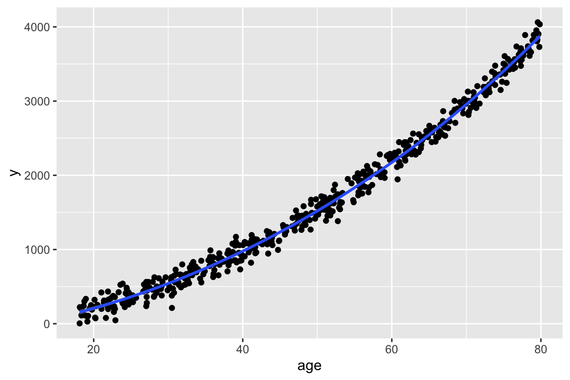

And let’s say we see the following plot for age-squared:

ggplot(df, aes(x = age_sq, y = y)) + geom_point() + geom_smooth()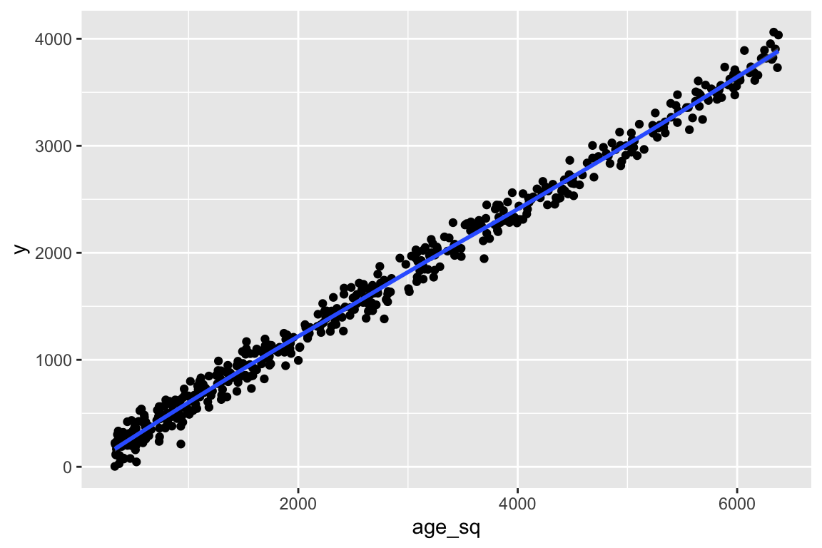

Then we would make the transformation of age for our model. When we include age-squared in the model, we still need to include age. We can run the model with both:

mod = lm(y ~ age + age_sq, data = df)

And we can look at the regression table. Notice that the standard error of age and age-squared’s coefficients are okay, but the intercept’s standard error is really big.

tidy(mod, conf.int = T) %>% gt() %>% fmt_number(decimals = 2)

term	estimate	std.error	statistic	p.value	conf.low	conf.high
(Intercept)	−56.66	34.92	−1.62	0.11	−125.27	11.96
age	2.29	1.54	1.49	0.14	−0.74	5.31
age_sq	0.58	0.02	37.80	0.00	0.55	0.61

We can also look at the VIF:

rms::vif(mod)

     age   age_sq 
37.01798 37.01798 

car::vif(mod) # will only give us GVIF if there is a multi-level covariate in the model

     age   age_sq 
37.01798 37.01798 

The VIFs are really big, so centering age will help the multicolinearity of the model.

mod2 = lm(y ~ age_c + age_c_sq, data = df)

Where age_c is age centered at the mean, and age_c_sq is the centered age squared.

tidy(mod2, conf.int = T) %>% gt() %>% fmt_number(decimals = 2)

term	estimate	std.error	statistic	p.value	conf.low	conf.high
(Intercept)	1,447.76	6.69	216.39	0.00	1,434.62	1,460.91
age_c	59.31	0.25	234.40	0.00	58.81	59.81
age_c_sq	0.58	0.02	37.80	0.00	0.55	0.61

car::vif(mod2) # will only give us GVIF if there is a multi-level covariate in the model

   age_c age_c_sq 
 1.00124  1.00124 

Yay! The VIFs are much better now! And the intercept and age coefficient estimate have better standard error!