Week 6

Categorical Covariates + Interactions

Room Locations for the week

• On Monday, 2/12,        we will be in virtual
• On Wednesday, 2/14,  we will be in RLSB 3A003 A

Resources

Lesson	Topic	Slides	Annotated Slides	Recording
10	Categorical Covariates
11	Interactions

On the Horizon

• Homework 3 due 2/15
• President’s Day on 2/19 (no class)
• Quiz 2 due 2/21
• Homework 4 due 2/22

Class Exit Tickets

Monday (2/12)

Wednesday (2/14)

Announcements

Monday 2/12

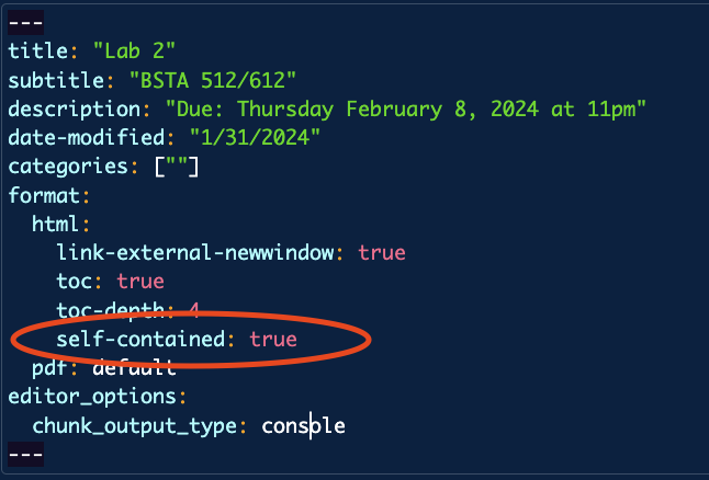
• Lab 2: please resubmit with self-contained: true

  • The top of your file should have the following line:

• Quiz 2 next week

  • Lesson 4 (SLR: Inference, starting at mean response) to Lesson 9

  • HW 4 will not be on it!

Wednesday 2/14

• Midterm feedback!!

  • Please complete by next Friday 2/23

  • Completely anonymous!

  • A question at the end will take you to another survey to record your name

Muddiest Points

1. Why do we need to create a new variable for ordinal / scoring?

Otherwise R will treat income as non-ordinal, and use the default reference cell coding. So if we want our variables to be scored (and numeric) then we must put it in a form R can recognize.

2. I’m a little confused on how the R code works for recoding/reordering our variables, specifically 1) why we use the mutate function but then use the same name for the variable/how that works and 2) why you need to include the list of each variable name in a vector. Basically, what each piece of that code does exactly and why it’s needed.

1. Mutate is just a function to create/change a variable. So if we are not fundamentally changing any aspect of the variable, we can call it by the same name. Helps keep our data frame neat by not tacking on additional variables.

2. When I am including the list of levels I am giving R the exact order to read each level. So if I want to go from high income to low income, I would reset the levels to the below code. Then R would read high income as the first level.

   gapm2 = gapm2 %>%
    mutate(income_levels = factor(income_levels, 
               ordered = T, 
               levels = c("High income", 
                          "Upper middle income", 
                          "Lower middle income", 
                          "Low income")))

3. Is there a rationale or strategy in choosing the most appropriate reference group?

Often no, not if the groups are not ordered. Things that you may consider:

• Is there a central group that you want to make comparisons to?

• Is there any social consequences of continually centering comparisons to one group? We may be consequentially centering the narrative around that group.

• When we interpret the coefficients, is there one group as the reference that makes it a little easier to interpret? (this has more of an effect in 513)

4. How do we build the regression indicators?

In R, we don’t need to build the indicators. If we have a variable that is a facotr with mutually exclusive groups, then R will automatically create the indicators within the lm() function.

5. Interpretations!

5.1 Interpreting a confounder

We model a confounder by adding it into the model (without an interaction, just the main effect).

• Thus, our interpretation follows the interpretations that were presented in Lesson 8: Intro to MLR

5.2 Interpreting the main effects when there is an interaction

Coming soon!!

5.3 Interpreting the interaction (effect modifier)

First, we model an effect modifier with an interaction!

Coming soon!!

6. Can we use continuous covariates in an interaction model?

Yes! Here are the four types of interactions we’ll discuss:

1. binary categorical and continuous

2. multi-level categorical and continuous

3. binary categorical and multi-level categorical

4. continuous and continuous

7. Synergerism vs. antagonism: how does \(\beta_3\) relate to each?

• Synergerism means the sign of interaction’s coefficient (\(\beta_3\)) matches that of main effect of \(X_1\), so the effect of \(X_1\) is strengthened as \(X_2\) increases

  • In the case that we’re looking at \(X_2\) as an effect modifier of \(X_1\)

  • It’s a little hard to think about this when we’ve only discussed \(X_2\) as a binary covariate, but our “increase” for an indicator is going from 0 to 1.

• Antagonism means the sign of interaction’s coefficient (\(\beta_3\)) is flipped from that of main effect of \(X_1\), so the effect of \(X_1\) is weakened as \(X_2\) increases

  • In the case that we’re looking at \(X_2\) as an effect modifier of \(X_1\)

  • It’s a little hard to think about this when we’ve only discussed \(X_2\) as a binary covariate, but our “increase” for an indicator is going from 0 to 1

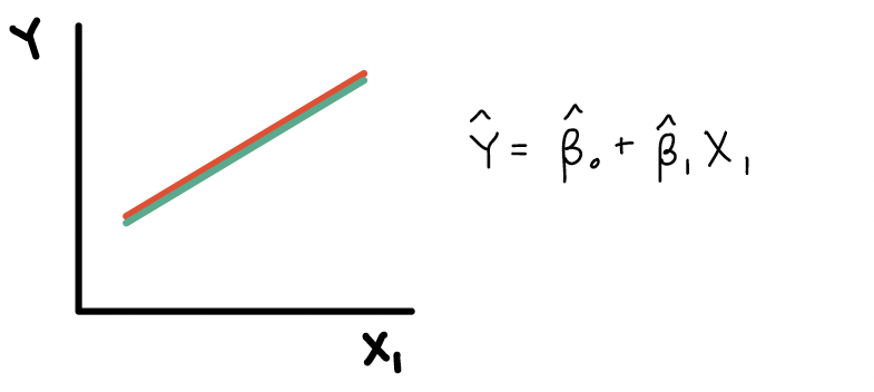
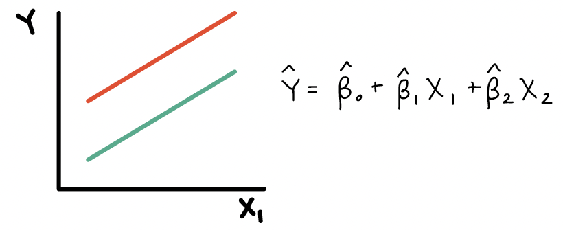
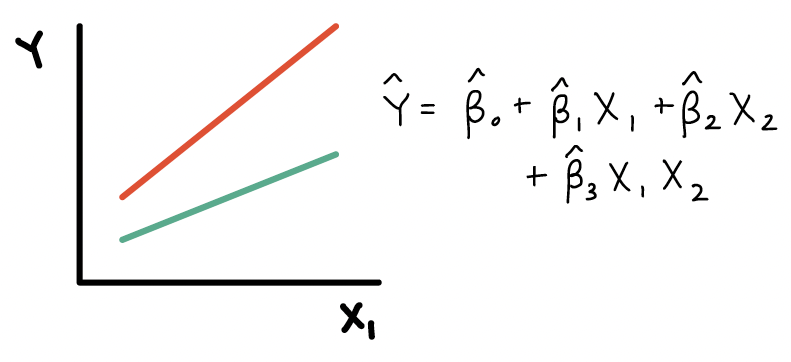
8. The red and green lines example. I’m not totally sure why the lines would be parallel if an interaction affects the slope of a line?

The lines should not be parallel if there is an interaction. Let me show the equation for each of those examples:

• Here is the plot and equation when \(X_2\) is a confounder:

  

• Here is the plot and equation when \(X_2\) is an effect modifier:

  

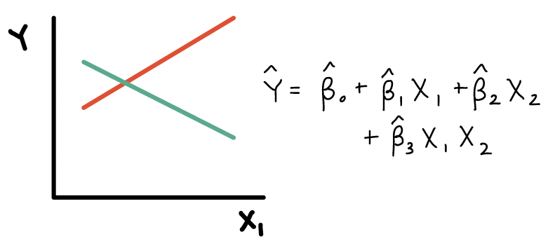
• Here is the plot and equation when \(X_2\) is a effect modifier:

  

• Here is the plot and equation when \(X_2\) should not be in the model: