Week 1
Resources
Below is a table with links to resources. Icons in orange mean there is an available file link.
| Chapter | Topic | Slides | Annotated Slides | Recording(s) |
|---|---|---|---|---|
| Intro | ||||
| 1 | Outcomes, Events, and Sample Space | |||
| 2 | Probability | |||
| 23 | Case Study on Counting |
For the slides, once they are opened, if you would like to print or save them as a PDF, the best way to do this is:
- Click on the icon with three horizontal bars on the bottom left of the browser.
- Click on “Tools” with the gear icon at the top of the sidebar.
- Click on “PDF Export Mode.”
- From there, you can print or save the PDF as you would normally from your internet browser.
On the Horizon
Class Exit Tickets
Additional Information
As we start the course, here are some administrative items that we need to do:
- Please join the Slack page
- Please read the syllabus on your own time
Extra Practice/Learning
- If you would like a Calculus review, please see this page!
- Combinatorics practice problems
- Pixar has a series of videos explaining how they use combinatorics in making animations
- This is a great & fun introduction to the basic principles of counting
- I highly recommend looking at them, especially if you have not studied permutations and combinations before.
- There is a table on p. 277 of the book with formulas for 4 different common counting cases (does order matter (y/n) vs. sampling with replacement (y/n).
- In class we covered all cases except “order does not matter and sampling with replacement.”
- This case is often referred to as the “stars and bars” problem.
- See this page for a proof to the Stars and Bars Theorem.
- Note: Their notation is opposite of what our textbook uses. The website uses k instead of n and n instead of r.
- In class we covered all cases except “order does not matter and sampling with replacement.”
Statistician of the Week: Regina Nuzzo

Dr. Nuzzo received her PhD in Statistics from Stanford University and is now Professor of Science, Technology, & Mathematics at Gallaudet University. Gallaudet University, federally funded and located in Washington, DC, is the only higher education institution where all programs are designed for the education of the deaf and hard of hearing. Dr. Nuzzo teaches statistics using American Sign Language.
She is the Senior Advisor for Statistics Communication and Media Innovation at the American Statistical Association and a freelance writer.
Topics covered
Dr. Nuzzo is a statistician and a science journalist. Her work has appeared in Nature, Los Angeles Times, New York Times, Reader’s Digest, New Scientist, and Scientific American. Most of her work is in the “Health” or “Science” sections of the aforementioned outlets. Primarily, she works to help lay-audiences understand science and statistics in particular. She earned the American Statistical Association’s 2014 Excellence in Statistical Reporting Award for her article on p-values in Nature. Her work led to the ASA’s statement on p-values.
Relevant work
- Nuzzo, R. “Scientific method: Statistical errors.” Nature 506, 150–152 (2014).
- Nuzzo, R. “Tips for Communicating Statistical Significance.” Science, Health, and Public Trust, National Institutes of Health, 2018.
- Nuzzo, R. “Vying for a soul mate? Psych out the competition with science.” Health: Features. Los Angeles Times, 2008.
Outside links
Please note the statisticians of the week are taken directly from the CURV project by Jo Hardin. I also invite you to check out this youtube video of her Women Rise Keynote address where she discusses her hearing impairment, career growth, and her work with p-values.
Muddiest Points
1. Why is the number of possible events \(2^{|S|}\)?
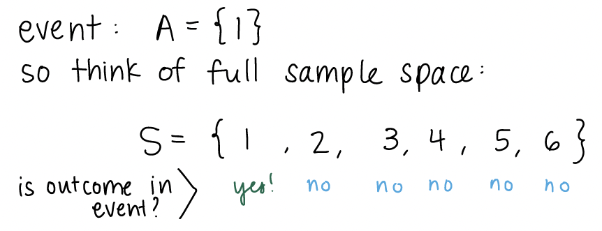
In class, we were wondering why/if \(2^{|S|}\) is the general formula for calculating the total number of possible events. We were specifically wondering if the \(2\) came from the fact that we had two options (heads and tails) for our outcome. Let’s work through the example of a 6-sided die to explain this further. The sample space is \(S=\{1, 2, 3, 4, 5, 6\}\). So is the total number of possible events \(2^6\) or \(6^6\) or something else? We can actually think about an event by using an indicator variable for each outcome of the sample space. An indicator variable is just a way to give us a yes/no answer to a question. So in this case, we are wondering: is this outcome a part of our event? If our event is \(\{1\}\) then for the outcome \(1\), the answer is “yes, the outcome is part of the event. For outcomes \(2-6\), the answer is”no, the outcome is not apart of the event.”
For each outcome, we have a “yes” or “no” answer. We can look at another example of an event. Let’s say our event is rolling an even number:
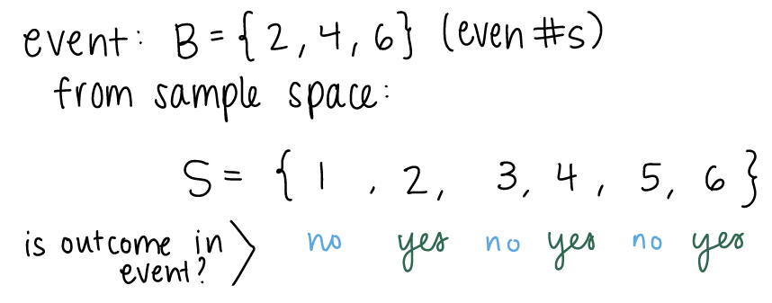
For \(2\), \(4\), and \(6\), the answer is “yes.” We can define the indicator variable for whether an outcome is in an event or not. The indicator gives a 1 or 0 for yes and no respectively.
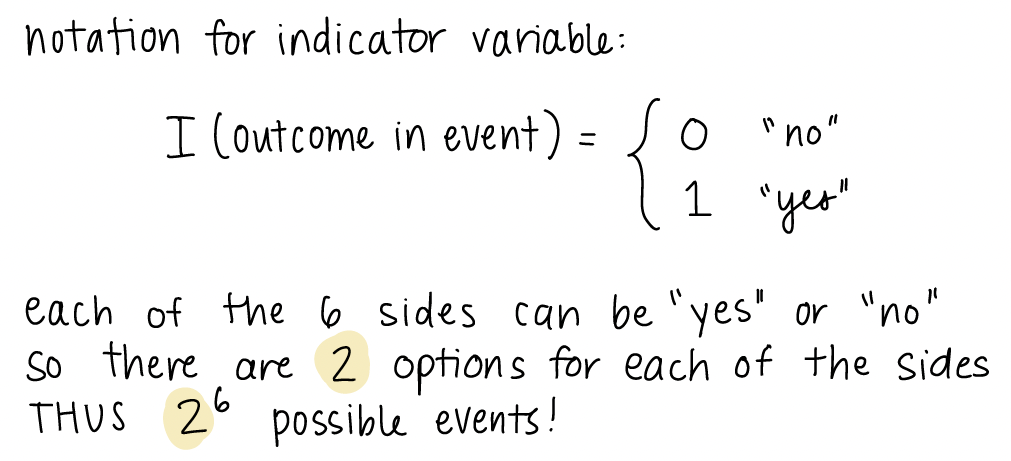
As stated above, the \(2\) in \(2^6\) comes from the \(2\) options from our indicator. Each side has two options, and there are \(6\) sides. Thus, \(2^6\) possible events.
2. What is an event??
I think this will become clearer when we start thinking about events in the context of probability. When we think of events outside of probability, we may think of something we actually do or something that happens, like going to a concert or coming to class or missing the streetcar. In this case, we think of the event as the single thing (out of all the options) that actually occured. For example, if I’m taking the streetcar to class, I can think of two definitive options of what might occur: I miss the streetcar or I get on the streetcar. Only one of these things can occur, which I may call an event colloquially.
It is important to make the distinction with events defined within probability. Events are not necessarily a single thing that occurred. Instead it can be a collection of things that may occur. In the example of the streetcar, I can define my event to include both options. Thus, my event is that I make the streetcar or I miss it. Both of these things cannot happen simultaneously, but if I want to calculate the probability that I miss or make the streetcar, then it is helpful to have the event defined.
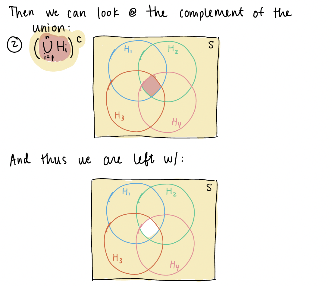
3. Confusion on the Venn Diagram for the high blood pressure example
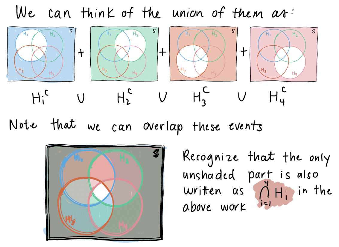
This is in reference to the Chapter 1 notes on “BP example variation (3/3)” slide. I explained the event that at least one subject does not have high blood pressure using a venn diagram. In this venn diagram, I assumed \(n=4\), and I wanted to show that the union of complements is equal to the complement of unions: \(\bigcup\limits_{i=1}^{n}H_i^C = \Big(\bigcap\limits_{i=1}^{n}H_i\Big)^C\).
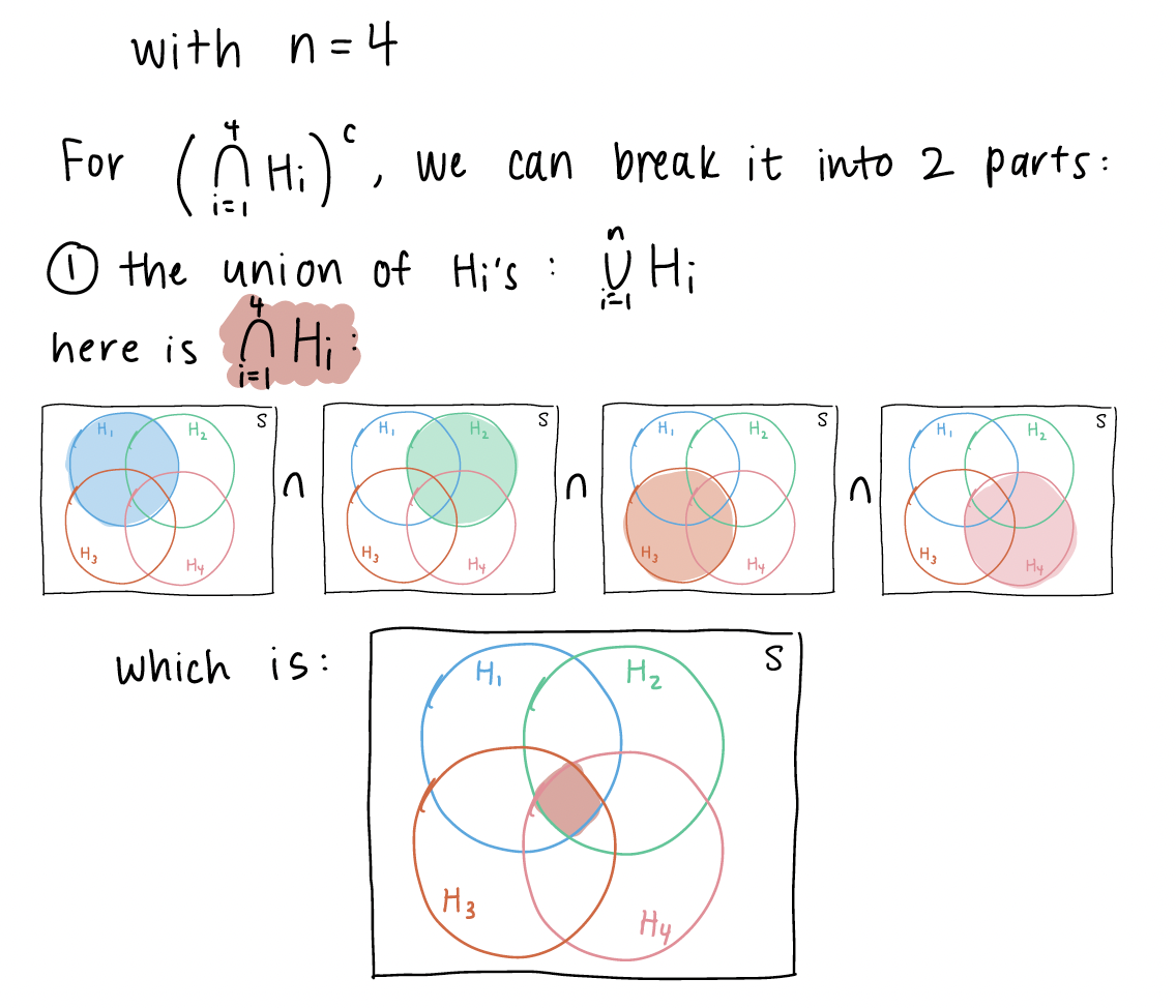
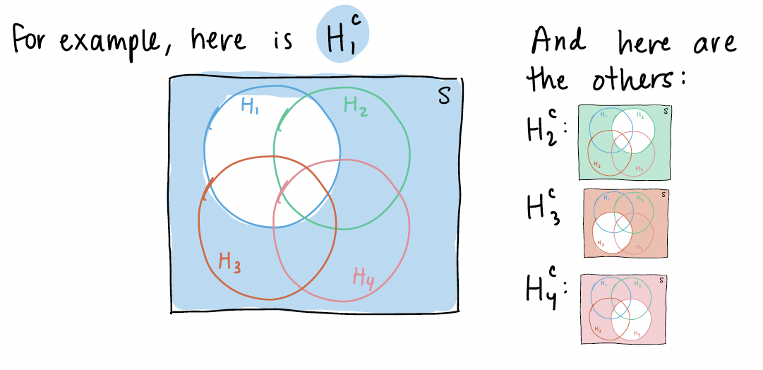
 Now we can look at \(\bigcup\limits_{i=1}^{4}H_i^C\). We first need to define \(H_i^c\)

4. Proofs of propositions
Further explanations of the propositions can be found in the textbook from pages 24-27. For many of the explanations in class, I was working to produce a union of disjoint events, so that the probability could easily be calculated. Proposition 3 and 4 were specifically mentioned, so I will include some writing notes on them here:
Proposition 3
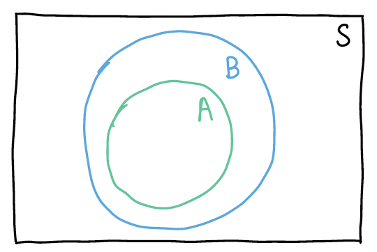
If \(A \subseteq B\), then \(\mathbb{P}(A) \leq \mathbb{P}(B)\)
In this proposition, I want to define event \(B\) as a union of disjoint events so that I can show \(P(B)\) is the sum of \(P(A)\) and some greater-than-or-equal-to 0 probability event. If the following is my venn diagram of A and B:
Then I can define B as the union of disjoint events: 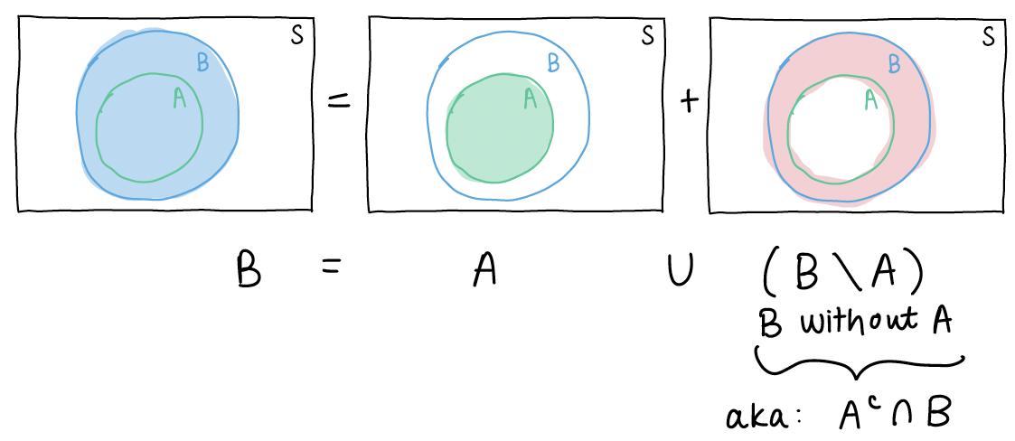
If we then take the probability of each side of the equation \(B = A \cup (A^c \cap B)\), we get \[P(B) = P\big(A \cup (A^c \cap B)\big)\]
Since events \(A\) and \(A^c \cap B\) are disjoint, the probability of their union is just: \[P(A) + P(A^c \cap B)\]
Thus, our equation is now \[P(B) = P(A) + P(A^c \cap B)\]
From Axiom 1, we know for event \(A^c \cap B\), \(P(A^c \cap B) \geq 0\).
So the probability of event B is the sum of the probability of event A and an event that is \(\geq\) 0. This means \(P(B) \geq P(A)\).
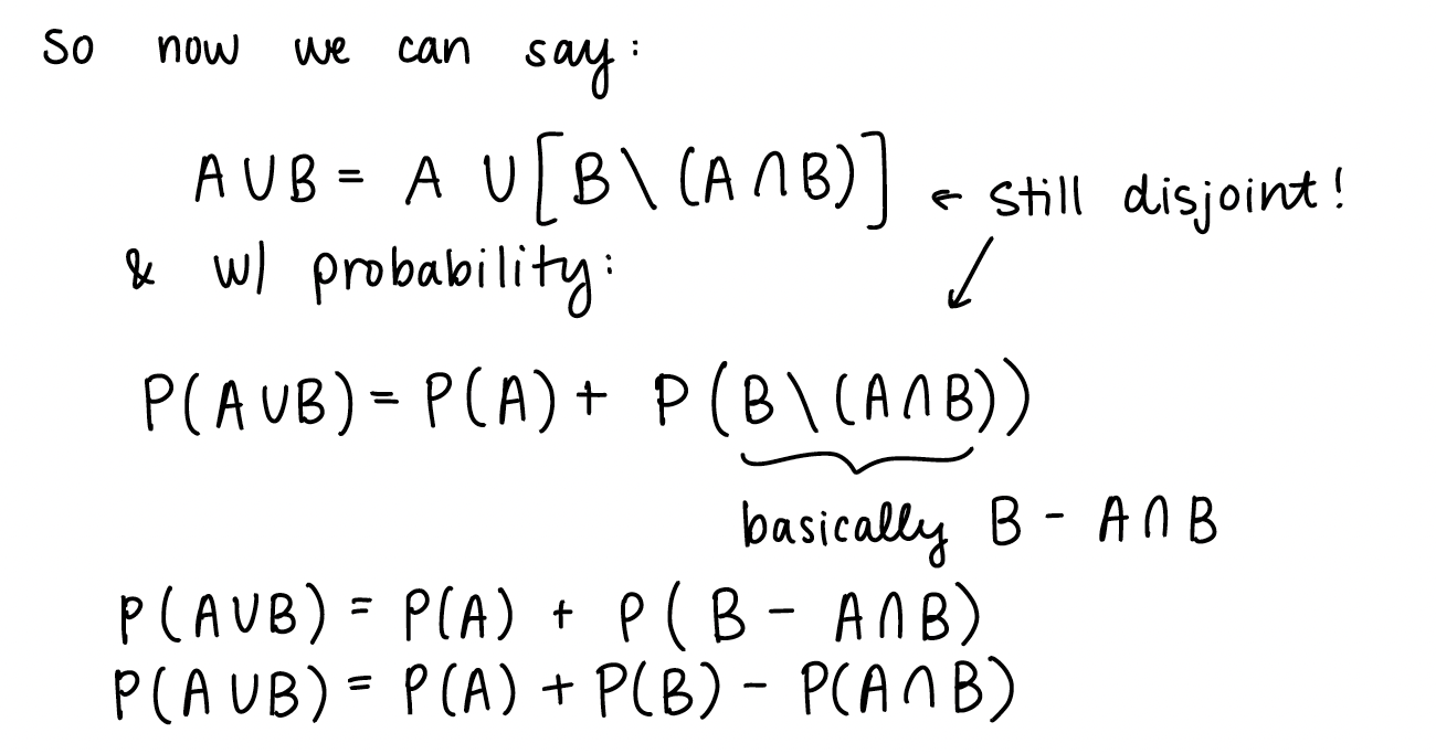
Proposition 4
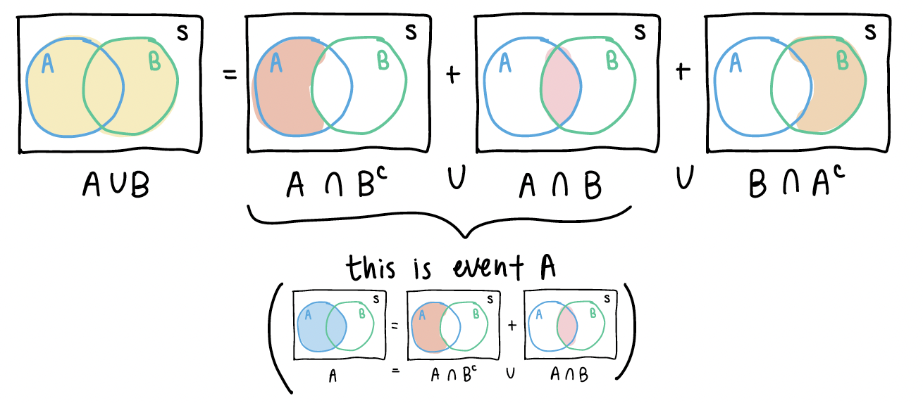
\(\mathbb{P}(A \cup B) = \mathbb{P}(A) + \mathbb{P}(B) - \mathbb{P}(A \cap B)\)
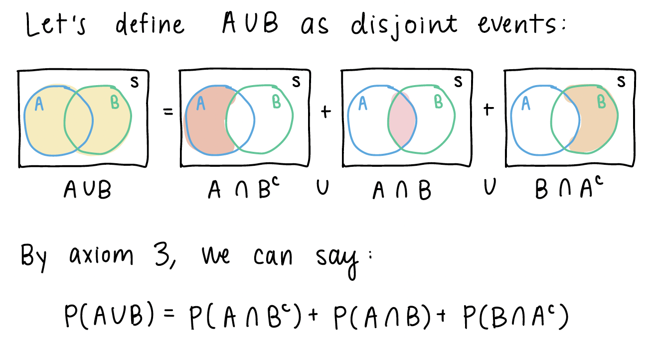
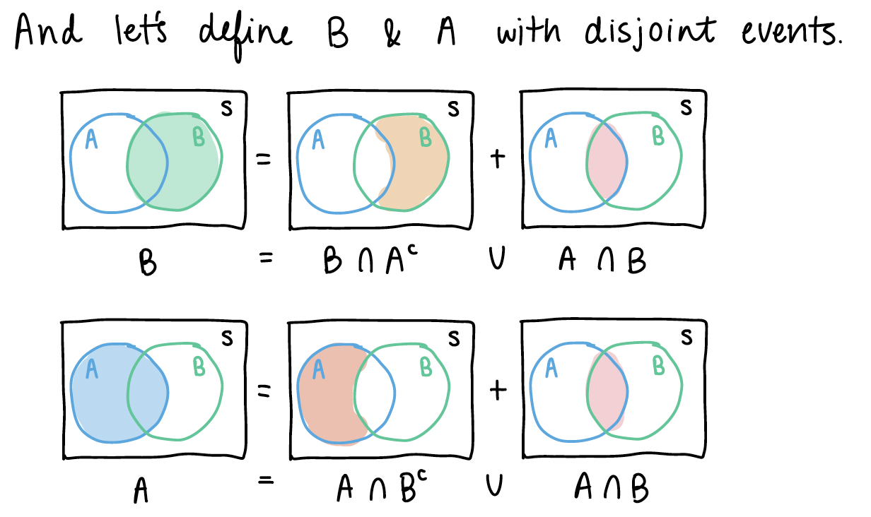
From the pictures above, we can see some similar disjoint events.
If we look back at \(A \cup B\), we can start manipulating the right side of the equation:

5. Example at end of Chapter 2 slides (Venn Diagram)
I will post this in the previous week’s Muddy Points as well. Please follow this link for my work through of the example. And here is the PDF with my work.
Sub-question: why don’t we just multiply the probability of A and B to get the intersection? This is a specific property of probability when A and B are independent. Only when A and B are independent can we conclude that \(P(A \cap B) = P(A)P(B)\).
6. Partition of events
We’ve been working with event partitions throughout Chapter 2, but we have not formally identified them. Partitions are advantageous to define for two reasons:
The partitions may be easier to calculate. We can then use the partitions to reconstruct other probabilities that may be more difficult to calculate
Partitions have nice properties as a consequence of being disjoint. For example, the probability of the union of partitions is the sum of the probabilities across each partition: \[P\bigg(\bigcup_{i=1}^n A_i\bigg) = P(A_1)P(A_2)P(A_3) \cdot \cdot \cdot P(A_n)\]
Clearest Points
Mostly: heads/tails example, sample space, how to draw a quarter, possible events for two coins.