Week 2
Resources
Below is a table with links to resources. Icons in orange mean there is an available file link.
| Chapter | Topic | Slides | Annotated Slides | Recording |
|---|---|---|---|---|
| 22 | Introduction to Counting | |||
| 3 | Independent Events | |||
| 4 | Conditional Probability | |||
| 5 | Bayes’ Theorem |
For the slides, once they are opened, if you would like to print or save them as a PDF, the best way to do this is:
- Click on the icon with three horizontal bars on the bottom left of the browser.
- Click on “Tools” with the gear icon at the top of the sidebar.
- Click on “PDF Export Mode.”
- From there, you can print or save the PDF as you would normally from your internet browser.
On the Horizon
Class Exit Tickets
Statistician of the Week: Talithia Williams

Dr. Williams earned a BS in Mathematics from Spelman College, an MS in Mathematics from Howard University, and a PhD (2008) in Statistics from Rice University. Dr. Williams is Associate Professor and Director of the Clinic Program at Harvey Mudd College. She has also served as Associate Dean for Faculty Development and Diversity at Harvey Mudd.
Topics covered
Dr. Williams works on statistical models which describe spatial and temporal aspects of data. Some of her most important work has focused on developing models to predict cataract surgical rates for countries in Africa.
Relevant work
Dray, A. and Williams, T. An incidence estimation model for multi-stage diseases with differential mortality. Statistics in Medicine, 2012.
Lewallen, S., Courtright, P., Etya’ale, D., Mathenge, W., Schmidt, E., Oye, J., Clark, A., Williams, T. Cataract Incidence in Sub-Saharan Africa: What does Mathematical Modeling tell us about Geographic Variations and Surgical Needs?. Ophthalmic epidemiology, 2013.
Outside links
Other
Dr. Williams was the co-host of the 2018 PBS Nova Wonders series.
Please note the statisticians of the week are taken directly from the CURV project by Jo Hardin.
Muddiest Points
1. Example at end of Chapter 2 slides (Venn Diagram)
I will post this in the previous week’s Muddy Points as well. Please follow this link for my work through of the example. And here is the PDF with my work.
Sub-question: why don’t we just multiply the probability of A and B to get the intersection? This is a specific property of probability when A and B are independent. Only when A and B are independent can we conclude that \(P(A \cap B) = P(A)P(B)\).
2. Partition of events
We’ve been working with event partitions throughout Chapter 2, but we have not formally identified them. Partitions are advantageous to define for two reasons:
The partitions may be easier to calculate. We can then use the partitions to reconstruct other probabilities that may be more difficult to calculate
Partitions have nice properties as a consequence of being disjoint. For example, the probability of the union of partitions is the sum of the probabilities across each partition: \[P\bigg(\bigcup_{i=1}^n A_i\bigg) = P(A_1)P(A_2)P(A_3) \cdot \cdot \cdot P(A_n)\]
3. Order matters vs. order does not matter
I think the best way to think about when order does and does not matter is through examples. So here is another example:
I randomly select 3 different people to be on my committee from a larger group of 5 people (we’ll call them people A-E) …
Order matters: If I want to assign each person to a specific role as I select them, then I want to keep track of the order
Order does not matter: If I just want to assemble a committee without any hierarchy, then the order that I select them does not matter
- So if I pick person A first, second, or third, they are still on the committee
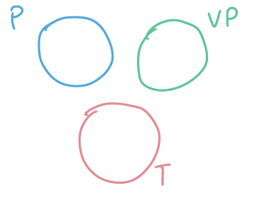
When order matters, the seats are now labelled as president, vice president, and treasurer:
When order does not matter, there are just three seats to fill:

For both situations, let’s say you pick person A, C, and E. When order matters, we can arrange these three people in a few ways:
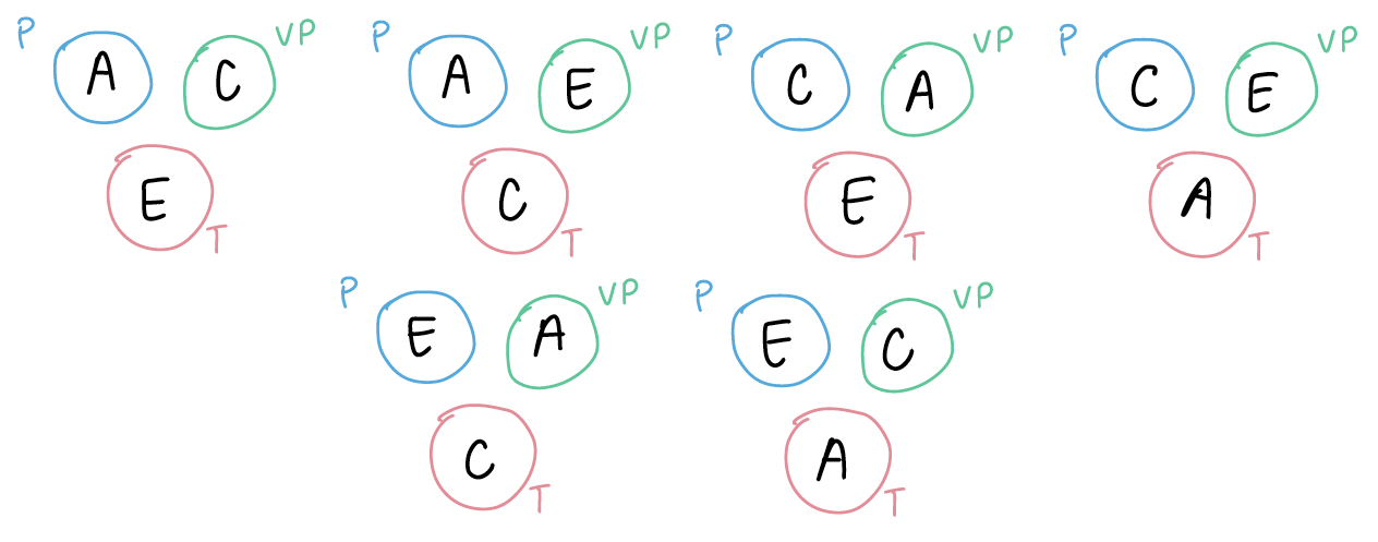
So there are 6 ways to order the three people.
When order does not matter, then we just need to know that person A, E, and C are on the committee:
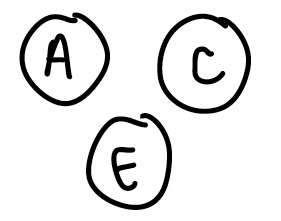
**Remember that there are 6 permutations to this 1 combination
Let’s answer more questions with this example…
When order does not matter, what are we controlling for?
In class example 1.3 and 1.4, we went from an example where order matters to one where order does not matter. So I showed us going from a calculation of \(\dfrac{10!}{4!}\) ways to order them to \(\dfrac{10!}{4!6!}\) ways of choosing 6 subjects. So why do we divide by \(6!\) when order does not matter? Let’s think back to our three committee seats. For the three seats, and person A, C, and E selected, there were 6 ways to order them. In fact, for any three people selected, there is always 6 ways to arrange (order) them into the positions. We can calculate the number of ways to arrange them with another permutation: if given three people and three seats, we can arrange them in \(3\cdot2\cdot1=6\) ways because we have three options for president, then once the president is selected, we only have 2 options for VP, then 1 for treasurer. So for every 6 ways to order the three people, there is only one way to select them unordered. Thus, we divide the number of ordered options by the number of ways each group of three people can be ordered.
So the calculation for the ordered committee (with P, VP, and T) is:
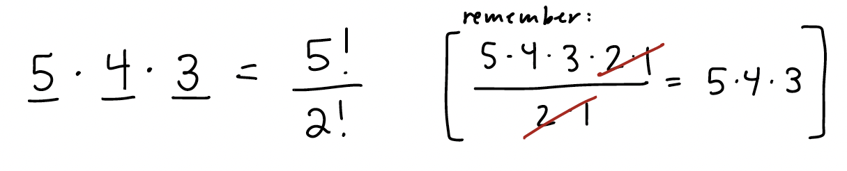
which is 60 ways to fill the committee seats when order (arrangement) matters.
And the calculation for the unordered (order does not matter) committee will divide the ordered permutations by the number of ways to order within the three seats:
which is 10 ways to fill the seats when order does not matter.
Is the probability equal when order matters and when order does not matter?
Yes and no…
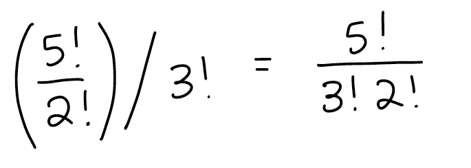
In the example with the spades, for order does not matter, we saw that \(r!\) cancels out and leaves us with a probability equal to when order does matter! This is because each spade is not distinguishable from the other. (Yes, technically each will have a different face, but we only care about the suit.) If we select a spade first then another spade, all we know of the order is spade first, spade second. If we flip that, we still get spade first, spade second. Thus, the order of the spades does not matter.
In the spades problem, we distinguished between “order matters” and “order does not matter” but the way we defined the probability, and the fact that spades are indistinguishable, means that the “ordered” cards really did not matter. It’ll definitely matter in an event where we get the first card as a spade and the second as a heart. We can no longer use combinations to define the event space!
The main take away should be that the probabilities (using order matters and order does not matter) are equal when order is not needed to define the event! When order does not matter, it can still be easier to calculate the probability using an “order matters” framework!! So we will use that to our advantage!
Below is some of the work demonstrating the probabilities loosely mentioned. Please note that ChatGPT could be a really helpful tool if you are curious about this question!
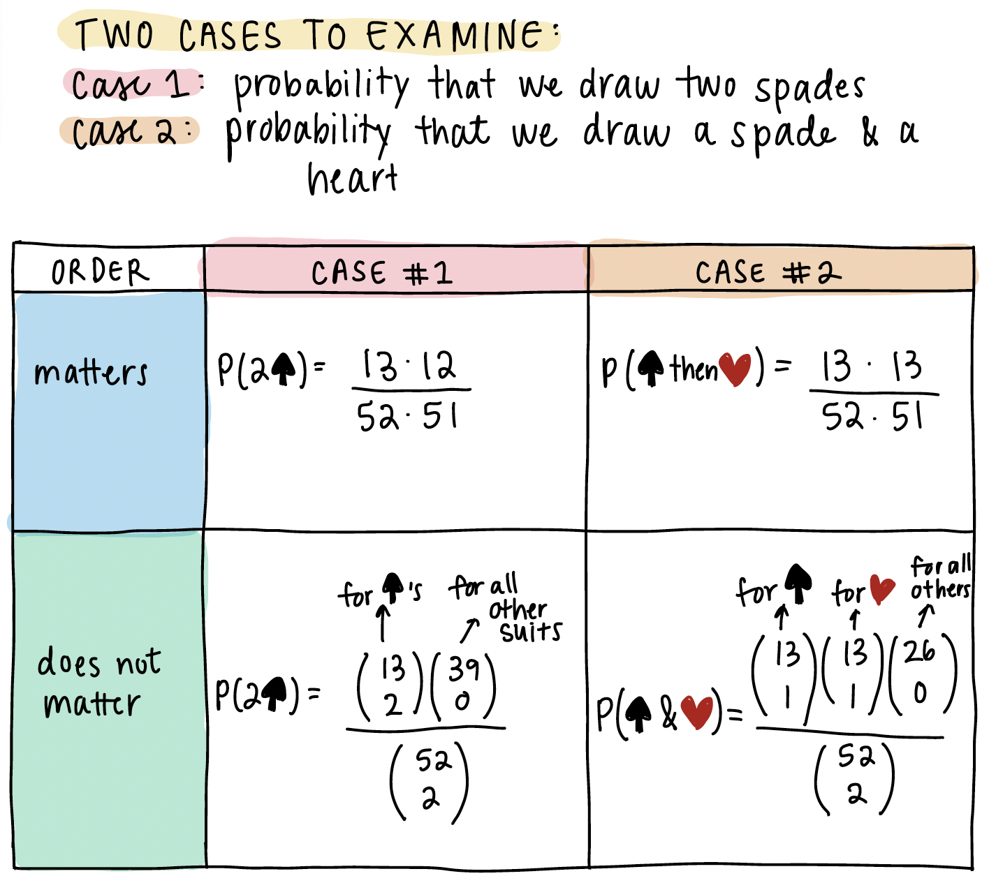
I’ll leave the work to calculate the exact probabilities above. For Case #1, the probabilities are equal. For Case #2, the probabilities are not equal!
4. Disjoint vs. Independent Events
Here is a pretty good video breaking down disjoint (mutually exclusive) events and independent events. It includes examples as well.
5. Conditional Probability Fact #4
Here is the 4th Conditional Probability Fact:
\(\mathbb{P}(A|B)\) is a probability, meaning that it satisfies the probability axioms. In particular, \[\mathbb{P}(A|B) + \mathbb{P}(A^C|B) = 1\] This is true even if A and B are NOT independent. Let me show you…
We can start by \(P(B)\) as the union of two disjoint events that involve \(A\) and \(A^c\):
\[ P(B) = P((A \cap B) \cup (A^c \cap B)) \]
Because they are disjoint, we can use Axiom 3 to say they are just the sum of each probability:
\[ P(B) = P(A \cap B) + P(A^c \cap B) \]
Now, we can divide both side of the equation by \(P(B)\):
\[ \begin{align} \dfrac{P(B)}{P(B)} = & \dfrac{P(A \cap B) + P(A^c \cap B)}{P(B)} \\ 1 = & \dfrac{P(A \cap B)}{P(B)} + \dfrac{P(A^c \cap B)}{P(B)} \\ \end{align} \]
By our definition of conditional probability, we know \(P(A|B) = \dfrac{P(A \cap B)}{P(B)}\) and \(P(A^c|B) = \dfrac{P(A^c \cap B)}{P(B)}\) Thus,
\[ 1 = P(A|B) + P(A^c|B) \]
Again, this is true even if A and B are NOT independent!