Week 8
Resources
| Chapter | Topic | Meike’s video | Slides | Annotated Slides | Recording |
|---|---|---|---|---|---|
| 25 | Joint Densities | ||||
| 26 | Independent continuous RVs | ||||
| 27 | Conditional distributions |
For the slides, once they are opened, if you would like to print or save them as a PDF, the best way to do this is:
- Click on the icon with three horizontal bars on the bottom left of the browser.
- Click on “Tools” with the gear icon at the top of the sidebar.
- Click on “PDF Export Mode.”
- From there, you can print or save the PDF as you would normally from your internet browser.
On the Horizon
Class Exit Tickets
Additional Information
Announcements 11/15
HW 5 feedback returned!
- Please look at the solutions for helpful R code!
HW 4 feedback
In NTB 1
Did not check all your numbers
Try to use variable name (like highest education level) when describing what the probabilities mean
NTB 4
Please relate this back to the hypergeometric distribution and see that each cashew drawn is not independent, but we get the same expected value as a binomial
As property of hypergeometric distribution (without replacement): expected value is the same as binomial (with replacement).
Final exam will not be cumulative
- Will only cover Chapter 24 and on
Student access to Vanport
- 5/6th floors: 7:30 a.m. to 9:30 p.m all days
Statistician of the Week: Desi Small-Rodriguez

Dr. Small-Rodriguez is a social demographer and an Assistant Professor of Sociology and American Indian Studies at UCLA. She received a PhD in Sociology from the University of Arizona and a PhD in Demography from the University of Waikato. Dr. Small-Rodriguez is Northern Cheyenne and Chicana and grounds her work in Indigenous studies, sociology of race and ethnicity, critical demography, and health policy research. She directs the Data Warriors Lab (a mobile data sovereignty lab serving Indigenous communities) and was previously a member of the Collaboratory for Indigenous Data Governance. She is a founding member of the Global Indigenous Data Alliance.
Topics covered
Dr. Small-Rodriguez is passionate about Indigenous data sovereignty and Indigenous data governance. Using networks of Indigenous scholars and survey methods, she works toward the following two goals: (1) better collection and use of data on Indigenous people that has been gathered by external sources such as the census and other federal entities; (2) development of data methods and practitioners within the Indigenous community. Dr. Small-Rodriguez also works for health and economic justice on Indian Reservations.
Relevant work
- S.R. Carroll, D. Rodriguez-Lonebear, A. Martinez, “Indigenous Data Governance: Strategies from United States Native Nations.” Data Science Journal, 2019. https://datascience.codata.org/article/10.5334/dsj-2019-031/
“Indigenous data sovereignty is the right of each Native nation to govern the collection, ownership, and application of the tribe’s data.”
- Rodriguez-Lonebear D, Barceló NE, Akee R, Carroll SR. “American Indian Reservations and COVID-19: Correlates of Early Infection Rates in the Pandemic.” J Public Health Manag Pract. 2020. doi: 10.1097/PHH.0000000000001206.
Outside links
Please note the statisticians of the week are taken directly from the CURV project by Jo Hardin.
Muddiest Points
1. How do pdf, CDF, and probability interact with each other?
Let’s say we have a pdf, \(f_X(x) = \dfrac{1}{9}x^2\) for \(0 \leq x \leq 3\). This is just a function. The pdf is not used on its own to report any probability. We must integrate over the pdf to find a probability.
Code
library("ggplot2")
eq = function(x){(1/9)*x^2}
ggplot(data.frame(x=c(1, 50)), aes(x=x)) +
  stat_function(fun=eq) +
  xlab("x") + ylab("pdf") +
  xlim(0,3)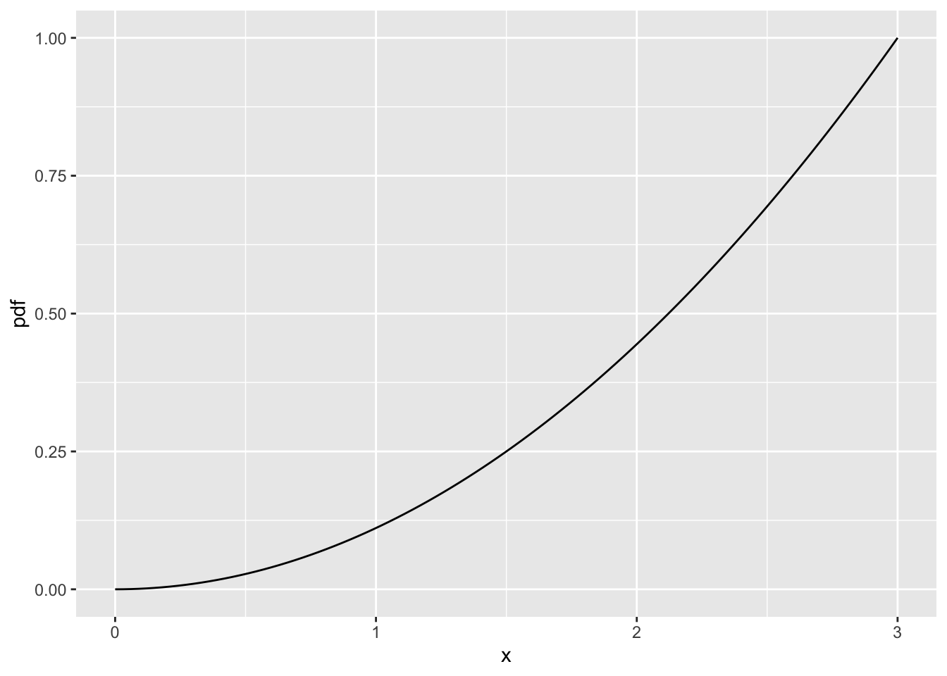
The total area under the pdf is 1. This makes our pdf valid.
Code
eq = function(x){(1/9)*x^2}
ggplot(data.frame(x=c(1, 50)), aes(x=x)) +
  stat_function(fun=eq) +
  xlab("x") + ylab("pdf") +
  xlim(0,3) +
  stat_function(fun=eq,
                xlim = c(0, 3),
                geom = "area",
                aes(fill = "red")) +
  theme(legend.position = "none") +
  annotate("text", x = 0.5, y = 0.7, label = "AUC = 1", color = "black")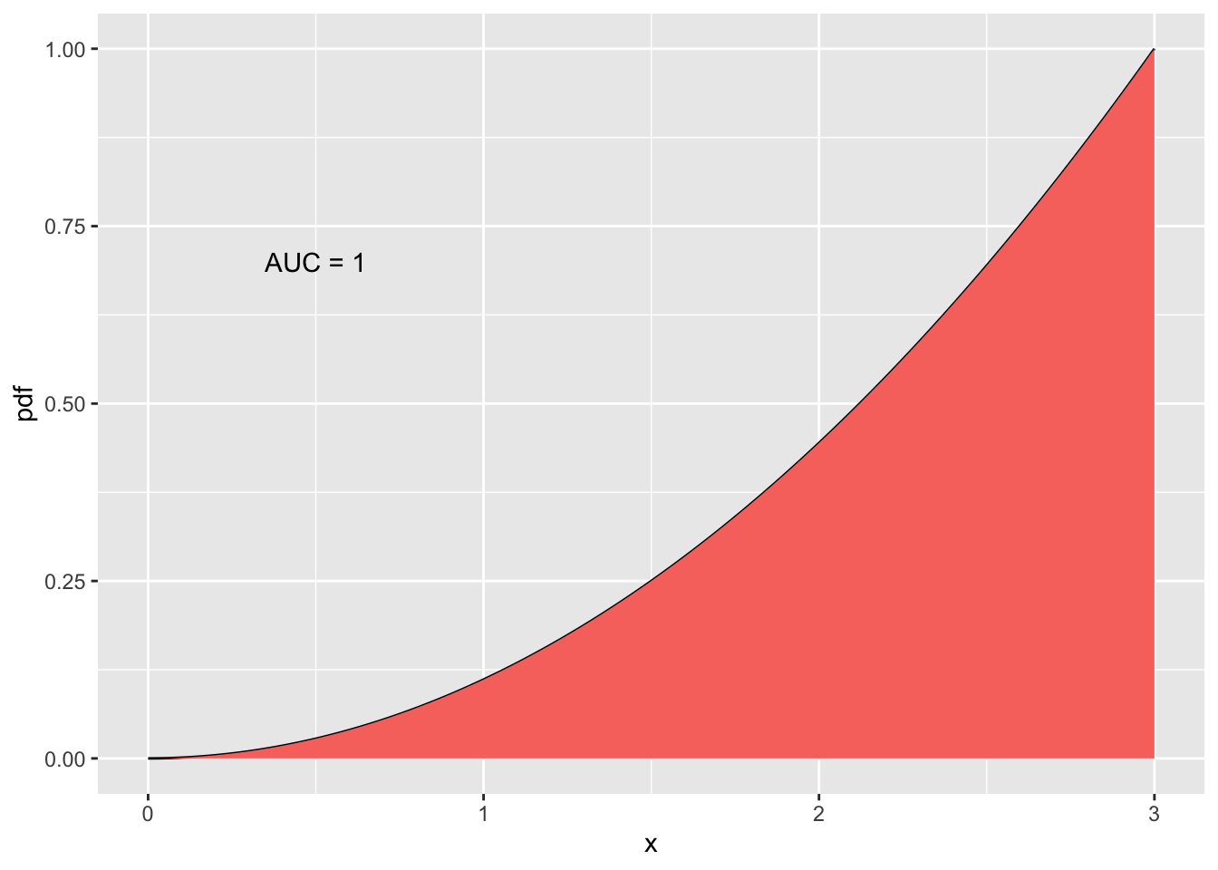
If we only look at a proportion of the area under the pdf, then we start constructing our probabilities. For example, we can look at probability that we have a value between 0 and 1.5.
Code
ggplot(data.frame(x=c(1, 50)), aes(x=x)) +
  stat_function(fun=eq) +
  xlab("x") + ylab("pdf") +
  xlim(0,3) +
  stat_function(fun=eq,
                xlim = c(0, 1.5),
                geom = "area",
                aes(fill = "blue")) +
  theme(legend.position = "none") +
  annotate("text", x = 0.5, y = 0.7, label = "AUC = 0.125", color = "black")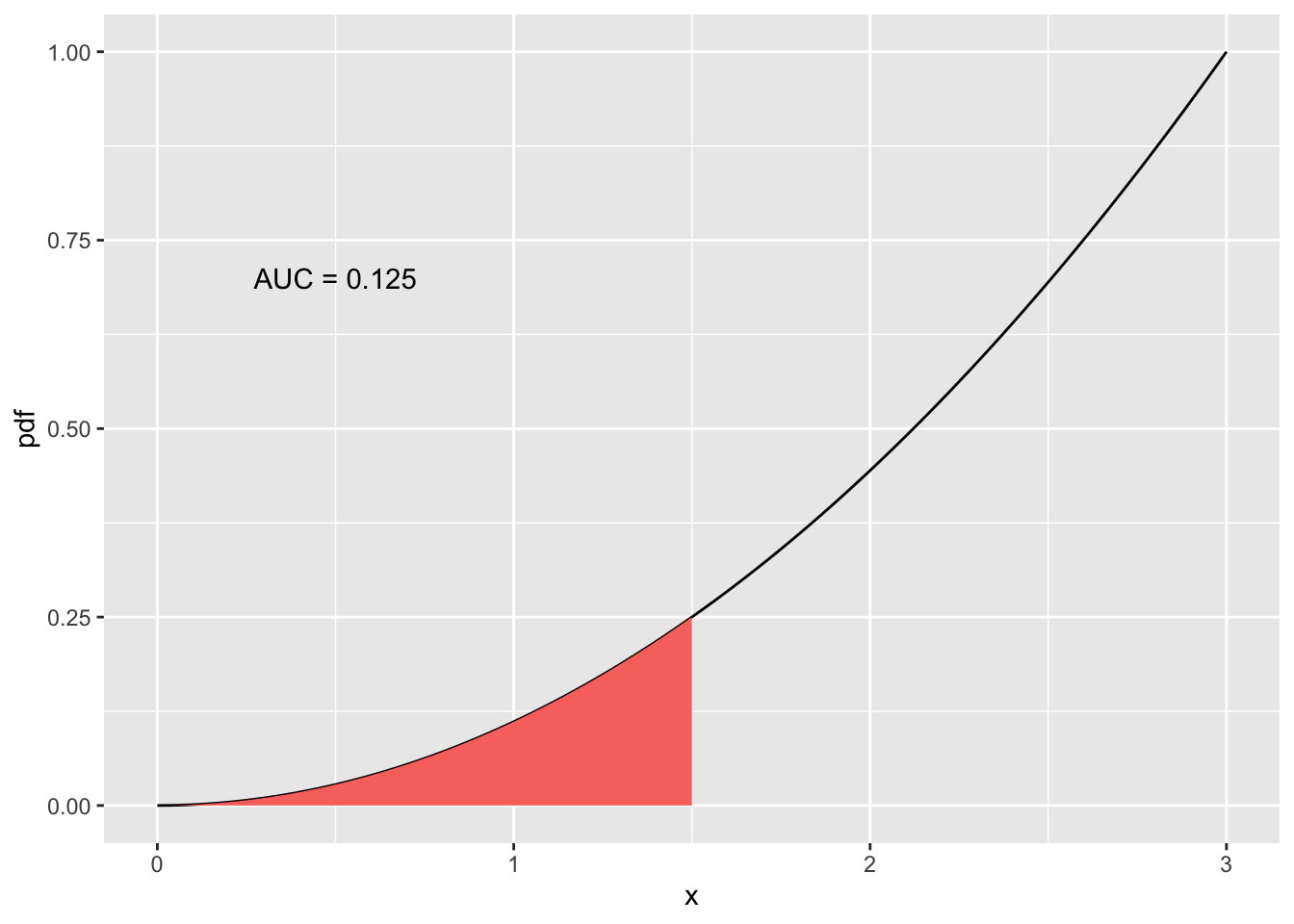
Instead of calculating the EXACT probability for each value between 0 and 3, we can find the CDF of the pdf.
The CDF is: \[ F_X(x) = \left\{ \begin{array}{ll} 0 & \quad x<3 \quad \\ \dfrac{1}{27}x^3 & \quad 0 \leq x \leq 3\quad \\ 1 & \quad x>3 \quad \end{array} \right. \]
Code
cdf = function(x){(1/27)*x^3}
ggplot(data.frame(x=c(1, 50)), aes(x=x)) +
  stat_function(fun=cdf) +
  xlab("x") + ylab("CDF") +
  xlim(0,3) +
  theme(legend.position = "none")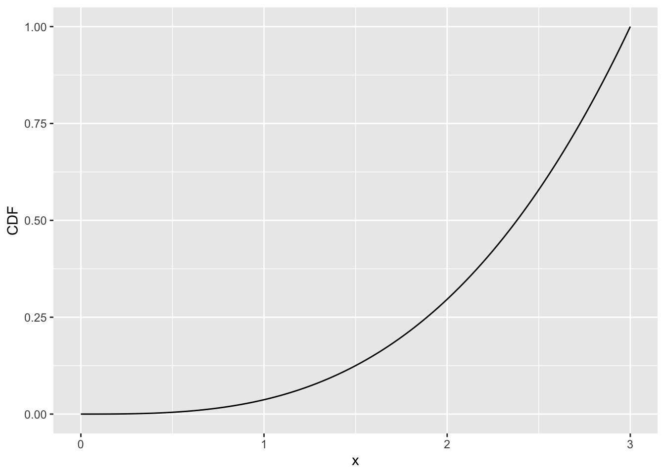
When \(x=1.5\), we can calculate the probability using the CDF. Remember that \(F_X(x) = P(X \leq x)\). So we can say \(P(X \leq 1.5) = F_X(1.5) = \dfrac{1}{27}(1.5)^3\), which equals 0.125.
Code
cdf = function(x){(1/27)*x^3}
ggplot(data.frame(x=c(1, 50)), aes(x=x)) +
  stat_function(fun=cdf) +
  xlab("x") + ylab("CDF") +
  xlim(0,3) +
  theme(legend.position = "none") +
  geom_point(aes(x=1.5, y=.125), colour="blue", size=3) +
  annotate("text", x = 0.5, y = 0.7, label = "CDF = 0.125", color = "black")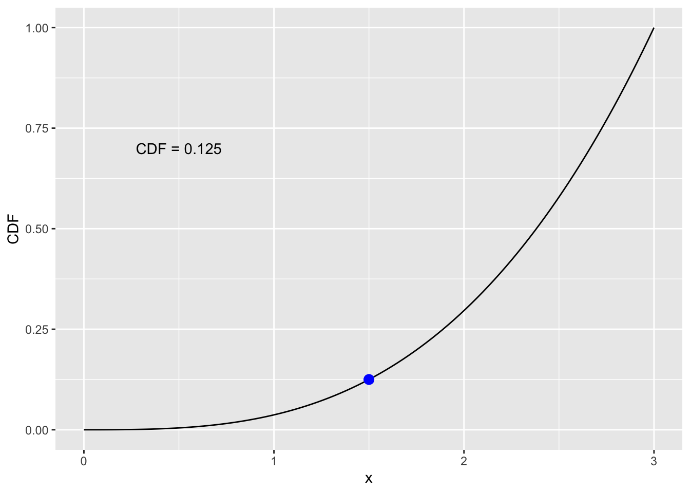
We can also calculate the probability with an integral: \(P(X \leq 1.5) = \displaystyle\int_0^{1.5} \dfrac{1}{9}x^2 dx\).
We can also find the probability that X is between two numbers. \(P(1\leq X \leq 1.5) = F_X(1.5) - F_X(1)\) or \(P(1\leq X \leq 1.5) = \displaystyle\int_1^{1.5} \dfrac{1}{9}x^2 dx\).
2. Joint vs marginal vs conditional: How are we calculating the probability?
If we start at a joint probability \(f_{X,Y}(x,y)\)…. we can look at a few probabilities:
Joint probability: \(P(a \leq X \leq b, c \leq Y \leq d)\)
\[P(a \leq X \leq b, c \leq Y \leq d) = \displaystyle\int_{x=a}^{x=b}\displaystyle\int_{y=c}^{y=d} f_{X,Y}(x,y) dydx\]
Marginal probability: \(P(a \leq X \leq b)\)
\[P(a \leq X \leq b) = \displaystyle\int_{x=a}^{x=b} f_{X}(x) dx\]
OR
\[P(a \leq X \leq b) = \displaystyle\int_{x=a}^{x=b}\displaystyle\int_{y=-\inf}^{y=\inf} f_{X,Y}(x,y) dydx\]
Conditional probability: \(P(a \leq X \leq b | Y = c)\)
\[P(a \leq X \leq b | Y=c) = \displaystyle\int_{x=a}^{x=b} f_{X|Y}(x|y=c) dx\]
You cannot calculate \(P(a \leq X \leq b | Y = c)\) by \(\dfrac{P(a \leq X \leq b, Y=c)}{P(Y = c)}\) because \(P(Y = c)\) is 0. Instead, we need to find \(f_{X|Y}(x|y=c)\) by \(\dfrac{f_{X,Y}(x,y=c)}{f_{Y}(y=c)}\) and THEN integrate over X.
3. What are we actually finding by solving the double integral. In the first example, we found the probability was 1/16 after integrating but what does 1/16 mean in relation to the random variables X and Y?
It means that the volume contained by \(0\leq X \leq 1\), \(0\leq Y \leq 1/2\), and their joint pdf is 1/16 of the total volume contained by \(0\leq X \leq 2\), \(0\leq Y \leq 1\), and their joint pdf. The probability for a joint pdf is now a measure of the proportion of the volume.
This is not be confused with a probability from marginal pdf or pdf from one RV. The probability for marginal/single RV pdfs is the proportion of the area under the pdf for a specific range of values.
4. Here’s a 3D plot of one of our joint pdf’s
\[ f_{X,Y}(x,y) = 5e^{-x-3y} \text{ for } 0 \leq y \leq x/2 \]
Code
library(plotly)

x = seq(0, 5, 0.1)
y = seq(0, max(x)/2, 0.1/2)
fn = expand.grid(x=x,y=y)
fn$z = ifelse(fn$y<fn$x/2, 5*exp( (-1)*fn$x - 3*fn$y), NA)

z = matrix(fn$z, ncol = 51, nrow = 51, byrow = T)

fig <- plot_ly(x = x, y=y, z=z) %>% add_surface()

fig